
A Star-Identification Algorithm Based on Global Multi-Triangle Voting
1
The School of Electronic and Information Engineering, Xi’an Jiaotong University, Xi’an 710049, China
2
The Xi’an Institute of Optics and Precision Mechanics, Chinese Academy of Sciences, Xi’an 710119, China
3
The State Key Laboratory of Astronautics Dynamics, Xi’an Satellite Control Center, Xi’an 710043, China
4
The Beijing Institute of Remote Sensing Information, Beijing 100192, China
*
Authors to whom correspondence should be addressed.
Appl. Sci. 2022, 12(19), 9993; https://doi.org/10.3390/app12199993
Submission received: 12 August 2022
/
Revised: 30 September 2022
/
Accepted: 1 October 2022
/
Published: 5 October 2022
(This article belongs to the Section Aerospace Science and Engineering)
Abstract
:A star-identification algorithm aimed at identifying imaged stars in a “lost in space” scene, named the global multi-triangle voting algorithm (GMTV), is presented in this paper. There are two core parts included in the proposed algorithm: in the initial match part, triangle feature units are treated as vote units to find the initial match relationship via matching vote units and counting the vote number of each catalog star. During this step, the principal component analysis (PCA) method is implemented to reduce feature dimensions, and a two-dimension lookup table and fuzzy match strategy are utilized to promote database searching efficiency and noise tolerance. After acquiring the initial match results, a verification part is implemented to filter potential errors from initial candidates by the largest cluster method and output the final identification results. The proposed algorithm achieves a 98.6% identification rate with 2.0 pixels position noise and exhibits more robustness to position noise, magnitude noise, and false stars of different levels than the two reference algorithms used in simulations. In addition, our algorithm’s real-time performance is better than reference algorithms, but it requires a larger database.
1. Introduction
Attitude measurement devices are key for modern deep space tasks. Generally, star sensors supply arc-second attitude data, whose precise level is much higher than sun sensors, gyroscopes, or magnetometers [1,2], and are now widely utilized in orbiting satellites and interplanetary spacecraft [3,4].
During data processing in star sensors, the star-identification technique plays a decisive role in determining attitude when utilizing detected stars in an image. There are two working modes for star sensors: lost-in-space (LIS) and tracking [5]. When we turn on star sensors or miss attitude data, the working mode of sensor stars will be in LIS, in which prior attitude data are absent, so an autonomous algorithm designed for whole sky identification is running to establish attitude data. Sky region information is acquired after determining the initial attitude in LIS mode, and then the star sensors switch to tracking mode and need to implement star identification in a very small sky region. Therefore, algorithm research about star identification in LIS is important for star sensors.
Star-identification methods for working in LIS mode can be divided into three classes [6]: pattern recognition, artificial intelligence, and subgraph isomorphism.
In the pattern recognition methods, each guide star is assigned a unique signature or pattern that describes the geometric distribution feature of neighboring stars, and then identification is implemented by searching for a guide star in the catalog whose pattern is the most similar to a star pattern built from the captured star image. The grid algorithm [7] is the most typical pattern-based approach utilizing a grid pattern vector, but its performance in the identification rate is sensitive to noise due to the low probability of selecting the correct subaltern star. Although some optimal schemes are introduced in [8,9,10], the key drawback in the grid algorithm has not been resolved. Zhang et al. [11] present a pattern recognition method utilizing radial and cyclic pattern features by adding a cyclic feature to filter error candidates. Unfortunately, the cyclic pattern is also not reliable enough. By optimizing the generation steps of a cyclic pattern, star identification based on radial and dynamic cyclic patterns is proposed in [12], where the maximum cumulate method is utilized to measure the similarity between cyclic patterns. However, the star-identification rate is prone to be low when there is magnitude noise. There are also other pattern-based algorithms proposed to improve robustness, such as the recommended radial pattern [13], log-polar transform [14], redundant-coded pattern [15], label code [16], and triangle map matrix methods [17], but their performance is still poor when there is magnitude noise.
Recently, artificial intelligence algorithms, especially those utilizing deep learning methods have been proposed for solving the LIS problem for star sensors. These include the Spider-CNN algorithm [18], RPNet algorithm [19], and 1D-CNN algorithm [20]. These algorithms have the parallel ability to process information and robustness to different types of errors, but considering the database size, the complexity of the model, and training time, these factors limit the application of deep learning methods in actual projects.
In subgraph-isomorphism-based methods, stars in the captured image and the angular distances between them are regarded as graph vertices and graph sides, respectively. Then, a feature subgraph unit for the matching process is built to search for similar subgraphs stored in the database, including entire sky graphs. The triangle algorithm [21,22,23], pyramid algorithm [24], and geometric voting algorithm [25] are typical star-identification methods based on subgraph isomorphism, in which polygons, pyramids, and star pairs are used as feature subgraph units. The triangle algorithm usually selects at least three true stars to generate some triangles and uses the angular distance or intersection angle of the graph sides as match elements. However, redundant or error matches of feature units in these methods often appear especially with noise, and their database size is also large. Several optimization strategies are presented to refine triangle algorithms in three terms: (1) the unit construction scheme, such as DUDE and the Delaunay principle introduced in [26] and [27]; (2) searching efficiency, for example, K–L transform [28] and hash map [29] methods proposed by Zhao and Wang to reduce the search dimension; and (3) verification reliability, such as the reference map verification method by Zhang presented in [21] to eliminate the error identification result. However, substantive defects of triangle algorithms are still not corrected due to the low dimension of the feature unit. By adding an extra star in the feature unit of a triangle, the pyramid algorithm utilized four stars to build a geometric polygon, named the pyramid feature unit, with six angular distances. Moreover, the k-vector approach is adopted to accelerate the matching efficiency of the high-dimensional feature unit, and it is proven to be robust to false stars. However, the pyramid algorithm becomes time-consuming when false stars are used to generate a feature unit. Kolomenkin et al. [25] presented a geometric voting technique by counting angular distance votes to determine the match relationship between image stars and guide stars. The real-time performance of this algorithm is acceptable when a few false stars exist but severely degrades with more spikes or false stars.
To improve the performance of the star-identification algorithm in LIS mode, a novel star-identification method utilizing a global multi-triangle voting (GMTV) scheme is proposed in this paper. Several triangle units are built by sensor stars as feature match units to determine the initial match relationship by matching these vote units and counting the number of votes of catalog stars, and then the initial results are filtered by a verification step based on the largest cluster method to remove errors and retain correct identification results as the final output. In addition, the principal component analysis (PCA) method is implemented to reduce feature dimension, and a 2D lookup table is also designed to accelerate searching efficiency in the initial match. The algorithm performs much better than the geometric voting algorithm and the grid algorithm in the presence of star position noise, magnitude noise, and false stars.
The rest of this paper is divided into the following sections: in Section 2, details of algorithm steps, including the initial match part and verification part, are presented. In Section 3, simulations are carried out to test the proposed algorithm’s performance in terms of the identification rate and efficiency and show the comparison results with two typical reference algorithms. In Section 4, key conclusions are given.
2. Algorithm Description
In this section, we describe the GMTV in detail. The triangle unit built by stars sharing the same field of view (FOV) is first introduced, and then the calculation of feature values representing the triangle unit is given. After, we construct the onboard database for the GMTV algorithm. Finally, the steps of the algorithm are described to illustrate the working principle of the GMTV algorithm.
2.1. Triangle Unit and Feature Extraction
The GMTV algorithm utilizes triangle units built by several bright stars in FOV as the basic match element and then extracts their feature values using the PCA method, which is the foundation of searching for the matching unit and implements a voting scheme. Hence, the triangle unit building and feature values calculation are briefly described as follows.
As shown in Figure 1, any three stars sharing the same FOV can be selected to build a triangle unit, such as unit k, which consists of Star-a, Star-b, and Star-c. By calculating the angular star distances between Star-a, Star-b, and Star-c, the triangle edge vector F of unit K can be obtained as Equation (1)
where adab, adac, and adbc are star angular distances between Star-a and Star-b, Star-a and Star-c, Star-b and Star-c, and adab < adac < adbc. The PCA method is then utilized to calculate feature values of triangle edge vector F to reduce feature dimension while retaining the main distinguishing features, as described in Equation (2).
[pv1, pv2, pv3] = PCA(F)
Feature values extracted by PCA are invariant to rotation and robust to noise. In this paper, we select pv1 and pv2 with larger values to keep unit geometric feature information. By utilizing the PCA method, a 1 triangle edge vector F is transformed into two feature values pv1 and pv2. After obtaining pv1 and pv2, we then discretize them in Equation (3), and the discretized feature values and are employed as the index to obtain candidates stored in the lookup table in the initial match step of GMTV.
where fix(x) returns the nearest integer value, which is no more than x, and u1 and u2 are discretized units of , respectively.
2.2. Onboard Database Generation
Figure 2 shows the database structure in GMTV, which consists of two parts, namely, the reference catalog and the triangle unit database, including the unit index table and lookup table, and occupies a 1.5 MB memory size.
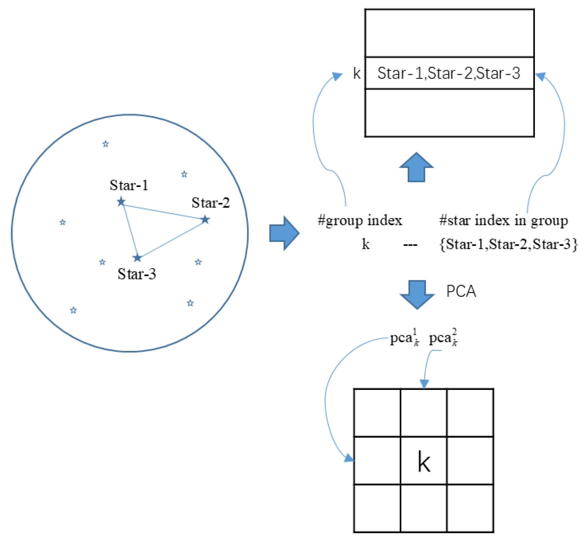
In this paper, the SAO J2000 catalog is selected as a basic catalog to build a database for the algorithm. After discarding the variable stars and binary stars from catalog stars whose magnitude value is down to 5.5 Mv, the reference catalog and unit index table of the database are first generated, and then feature values of each unit are calculated and stored in the corresponding index position of the lookup table. Considering the memory size and redundant matching probability, we only choose some triangle units as vote units in the GMTV database. Detailed steps about building the reference catalog and lookup table are described as follows: the whole celestial sphere is scanned uniformly with steps, namely, the right ascension angle of FOV is varied from 0° to 360° in steps of 0.5 degrees, and the declination angle of the FOV from −90° to +90° in steps of 0.5 degrees, and for each FOV at a different orientation, the brightest detected stars in the FOV are selected as guide stars and added to the reference catalog ( in this paper). After determining the guide stars in an FOV, we build triangle units by choosing any three stars from guide stars, so there are triangle units. During the above process, the indexes of the three stars in the SAO for each triangle unit are stored as a group in the unit index table, and the feature values of the unit are stored in the 2D lookup table; the process above, for example, is illustrated in Figure 3.
In Figure 3, a triangle unit whose unit index is K consists of three catalog stars, whose star index is Star-1, Star-2, and Star-3 in the SAO catalog, and its feature value is and . Thus, Star-1, Star-2, and Star-3 are stored in the Kth row of the unit index table, and unit index K is stored in the position of the lookup table where the row index is and the column index is .
2.3. Global Multi-Triangle Voting Algorithm
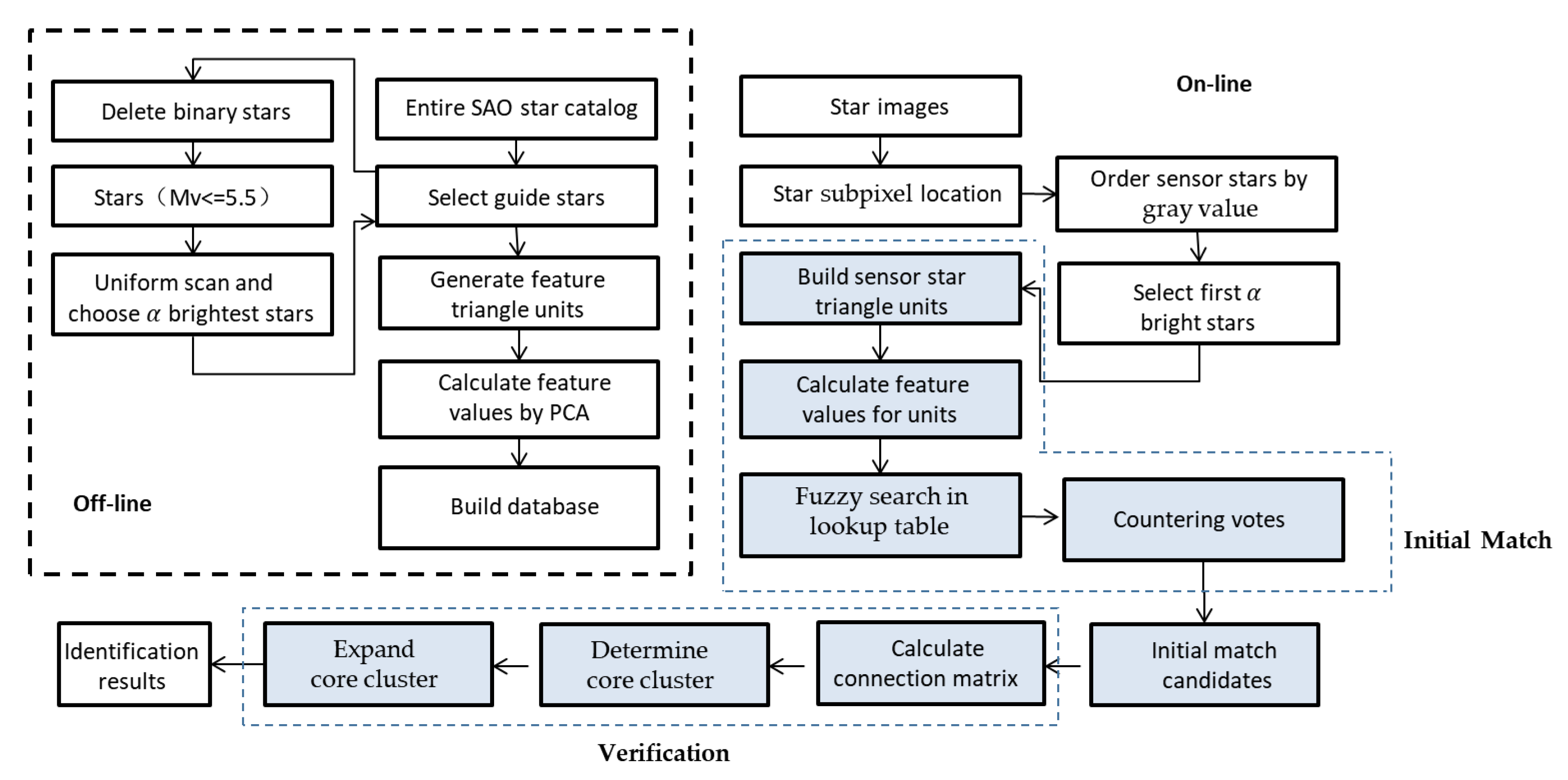
After extracting the stars in the observed image, the information data about the subpixel coordinates and gray values of the stars in the image plane are acquired and inputted to the GMTV algorithm. Then, the GMTV obtains some candidates of these captured stars by matching the triangle units and voting for the catalog stars. The catalog stars whose counter values are larger than the threshold are chosen as candidates for the detected stars. The correct catalog star is always included in the candidate set, but unfortunately, sometimes, there are errors because of noise. Therefore, we must design a filter process to select the correct catalog from the candidate set and remove incorrect matching results. The GMTV algorithm includes two steps: the initial match step using the voting global multiple triangle units and the verification step searching for the largest cluster. In the initial match step, feature values are calculated and then candidates are acquired by voting units. In the verification step, the largest cluster is searched to determine the final identification results as the output of the GMTV, as shown in Figure 4.
2.3.1. Initial Match
At the beginning of the initial match step, we select the eight brightest detected stars in the captured image as sensor stars to be identified according to their gray values, then a counter group (,…) including counters, is assigned for every sensor star, in which each counter is responding to each guide star in the reference catalog, and is the guide star number in the catalog. We can build triangle units from these bright sensor stars by selecting any three stars among them. As a result, there are units involved in the initial match. For each triangle unit, and values are acquired by the feature extraction process described in Section 2.1. Here, an example is given to illustrate the GMTV algorithm work process in this step.
We assume that unit k, including sensor star a, star b, and star c, is built, and its feature values and are also obtained. For database units whose feature value , (c = 1, 2, 3, …, N − 1, N, and N is the total number of triangle units) is close to the corresponding , , respectively, which can be described in Equation (4), these units in the database are considered as candidates of sensor unit k.
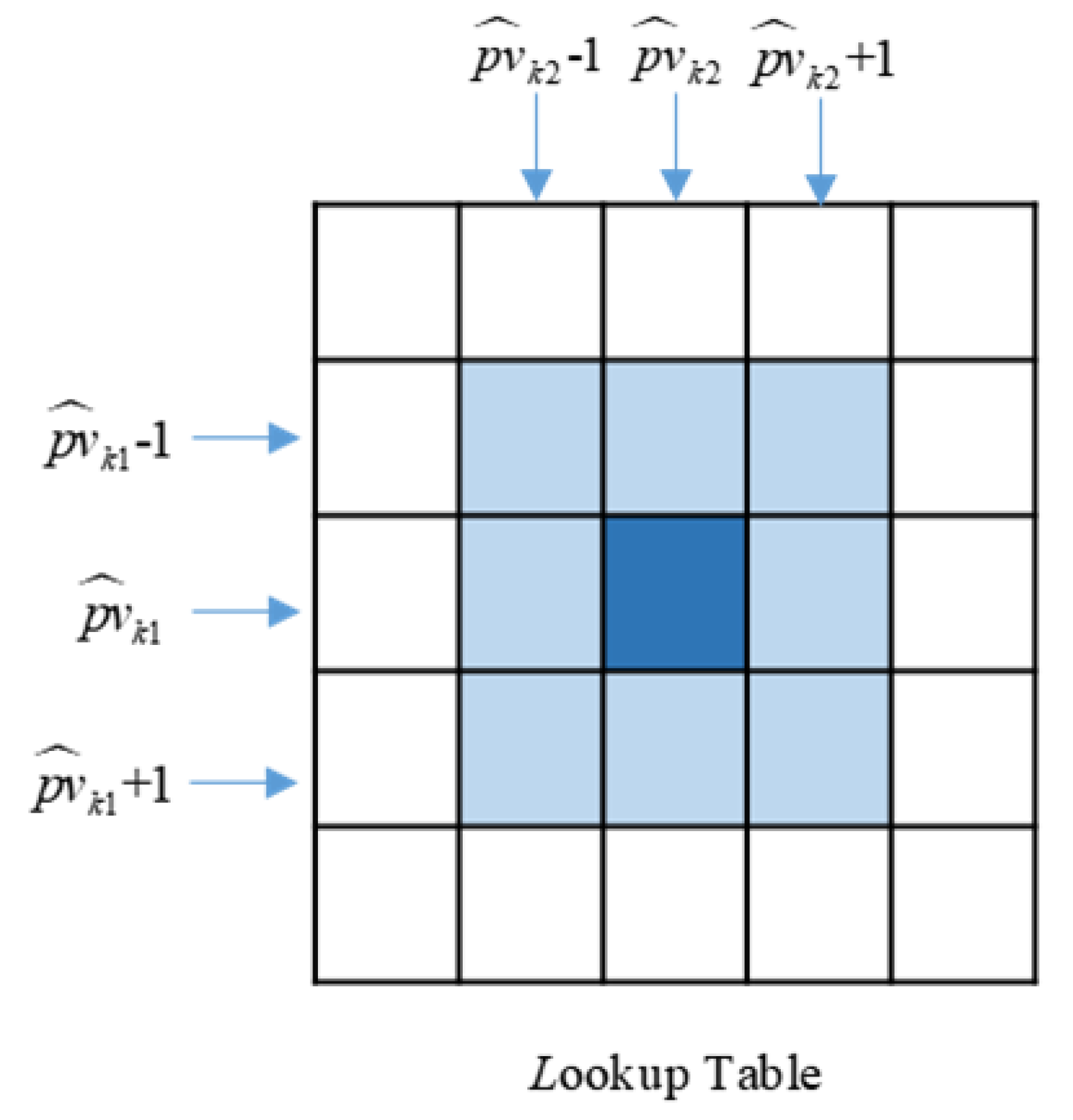
where is the threshold for the feature value match. The above candidates searching process can be implemented by looking for an element where the row index is and the column index is in the lookup table, which greatly improves the efficiency of the GMTV algorithm in searching for matches in the database. In the real star image, some measurement errors will cause feature values to deviate from their true value, so the fuzzy search strategy is adopted in our algorithm to increase robustness; as shown in Figure 5, all elements in the shaded areas whose position index is close to and , namely, where the row index is between − 1 and + 1 and the column index is between − 1 and + 1 simultaneously, are regarded as candidates of the sensor unit.
A unit in the lookup table constructed by catalog stars whose index number is C1, C2, and C3 in the SAO catalog is a candidate for sensor unit k (built by sensor star a, star b and star c). Then, the counter group belonging to the sensor star is selected, and the value of counters in (, …) corresponding to C1, C2, and C3 add one; as shown in Figure 6, is a counter assigned for guide star C in the counter group belonging to sensor star a (ssa), the same meaning of and . The same operation is completed for the other two counter groups belonging to sensor star b (ssb) and sensor star c (ssc), respectively. The above process is a vote of sensor unit k. We can repeat this voting process until all sensor units are traversed. For each sensor star, the counters’ values in the group are compared with the threshold Thc, and the catalog stars associated with counters whose values are larger than Thc are considered as the candidates for this sensor star.
2.3.2. Verification
In this paper, a verification method based on the largest cluster is designed to eliminate wrong candidates in the initial match, retain correct identification results as much as possible, and then output them as the final identification results of the algorithm. The maximum cluster verification algorithm includes three steps: calculate the connection matrix, determine the core cluster, and expand the core cluster. The specific contents of the above three steps are as follows:
Step 1: calculate the connection matrix
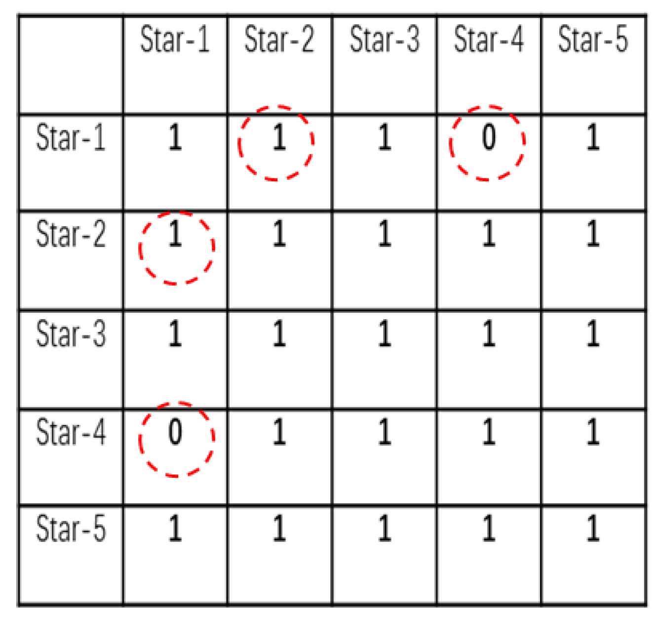
Calculate the angular distance between the candidate stars in the celestial coordinate system, and then compare with the angular distance of the corresponding observed stars in the star sensor coordinate system. If the error between and is less than a tolerance threshold , as described in Equation (5), the element in the corresponding position of the connection matrix is set to 1; otherwise, it is set to 0. The connection matrix is a square matrix of size DD, where D is the number of candidate stars in the initial match. For example, as shown in Figure 7, given that the angular distances between star-1 and star-2 meet the above requirement that the error between and is less than , then the elements in the position index (1, 2) and (2, 1) of the connection matrix are set to 1. Since the angular distances and between star-1 and star-4 do not meet the requirement of Equation (5), the elements in the position index (1, 4) and (4, 1) of the connection matrix are set to 0. It should be noted that the diagonal elements of the connection matrix are all set to 1.
Step 2: determine the core cluster
The determination of the core cluster step includes two main parts, namely, searching the initial largest cluster and filtering the initial largest cluster elements. The specific contents are as follows:
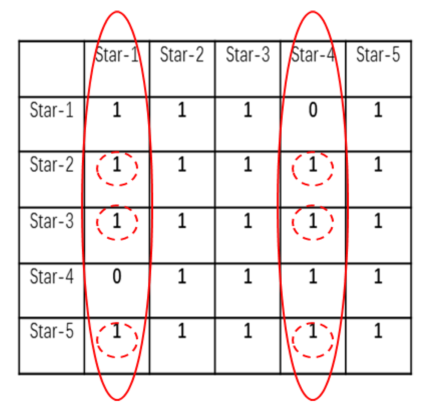
In the first part, the elements of the connection matrix are added in the column direction, the column with the largest summation value is determined, and then the candidate stars corresponding to the rows with the element value of 1 in this column are selected to generate the initial largest cluster. For example, as shown in Figure 8, the values after summing the elements in the column direction are 4, 5, 5, 5, 4, and 5, so the second column is of maximum value, and because its elements in rows 1 to 5 are 1, the initial largest clustering is {Star-1, Star-2, Star-3, Star-4, Star-5}.
In the second part, the elements in the initial largest cluster are filtered to determine the core cluster. As shown in Figure 9, * is the bitwise multiplication operator; we can bitwise multiply the corresponding column vector in the connection matrix where the initial largest cluster is located with the first column vector, and then bitwise multiply the result of the previous step with the second column vector, then repeat the same operation until the last column vector. Then, a column vector of size D1, defined as the filter vector, is obtained. Next, the candidate stars in the filter vector whose corresponding element value is 1 are selected in the core cluster. For example, the second column vector is bitwise multiplied by each column vector in the connection matrix, and the filter vector is [0 1 1 0 1]’, so the core cluster is {Star-2 Star-3 Star-5}.
Step 3: extend the core cluster
After determining the core cluster, the core cluster is utilized to search for more correct candidates not included in the core cluster due to noise to improve the attitude accuracy of the star sensor, but at the same time, it has to be ensured that wrongly identified results must be excluded. Based on the above principles, the candidate stars in the core cluster are selected as references to verify the remaining candidate stars. If all elements of the column vector of a remaining candidate star in the row position corresponding to candidates included in the core cluster are 1, then this candidate is considered as correct and included in the final identification result. Otherwise, it is not included. For example: star-1 and star-4’s column vector elements in rows 2, 3, and 5 are all 1 (as shown in Figure 10), so they are determined as correct identification results by the core cluster {Star-2 Star-3 Star-5}, so the final output is {Star-1 Star-2 Star-3 Star- 4 Star-5}.
3. Simulations and Results
Simulation experiments including different levels of position noise, magnitude noise, and different numbers of false stars have been completed to test the proposed star-identification algorithm. In this paper, the following two judgment conditions need to be met simultaneously for a successfully identified star image: (1) neither true stars are identified incorrectly, nor false stars are identified as a guide star. (2) more than two true stars are correctly matched in the identification result. Moreover, two classic star-identification algorithms belonging to different types were selected as comparison algorithms, namely, the geometric voting algorithm and the grid algorithm, because they have been proven to be excellent in several space missions, and we validated the proposed algorithm by comparing the identification rate, run time, and database size with these methods. In simulations, the key parameters of the star sensor are given in Table 1, and 9040 stars brighter than 6.5 Mv in the SAO J2000 star catalog were chosen to generate simulated star images. In addition, all the algorithms in this section were written in MATLAB R2021 and implemented on a personal computer with a Core 3.4 GHz.
3.1. Parameter Selection
Two discretizing parameters, and , have a significant impact on the identification rate, especially for star images with position noise. When there are position errors with a large deviation in an image, it is reasonable to set and to bigger values for more tolerance for noise. However, too many redundant guide stars may be matched as candidates to severely decrease the effectiveness of the voting process. However, when and are set to small values, there is a greater possibility that the correct candidates of the voting unit are eliminated.
The relationship between and the identification rate as the standard deviation of position noise increasing from 0 to 2.0 pixels is illustrated in Figure 11, while the standard deviation of the magnitude noise remains at 0.3 Mv. It can be seen that when position errors increase by more than 1.0 pixel, the algorithm performance degrades differently for different parameters groups, particularly for parameter group 1 and group 3, in which are set to 0.05 and and 0.015 and, respectively.
It is important to note that the algorithm achieves a higher identification rate of more than 97% with 2.0 pixels of noise in parameter group 2, where. Furthermore, the average run times are 16.24 ms, 18.36 ms, and 21.87 ms for parameter group 1, group 2, and group 3, respectively. Considering both the robustness to position noise and run-time performance of the algorithm, we selected parameter group 2 as the discretizing unit parameters in the paper.
3.2. Comparison and Analysis
The influence of the three different types of noise (position noise, magnitude noise, and false stars) on the identification rate of the proposed algorithm, geometric voting algorithm, and grid algorithm is shown in this section. The position noise added to the observed star makes the corresponding projected centroids deviate from their theoretical location coordination. Compared with the star magnitude data listed in SAO, there are some errors in the star brightness for images captured by the star sensor, which leads to some brighter stars, whose magnitude value in the star catalog is less than 5.5 Mv, being lost in star images, while dimmer stars, whose magnitude value in the star catalog is more than 5.5 Mv, are captured by the star sensor and appear in the image. Besides the above two measurement noise sources, false stars may appear in the captured image because planets, observed spacecraft, radiation, space fragments, and hot spots may also appear in the captured image, and these are mistakenly regarded as true stars. In our experiment part, all parameters of the algorithm are fixed, and one noise source increases linearly, while the others are maintained at a typical level. In total, 5000 star images are generated and identified by the three algorithms to evaluate their identification rates with different noise conditions through the Monte-Carlo method.
(1). Robustness toward star positional noise: Figure 12 illustrates the identification rates of star images for three algorithms when the star position noise increases linearly from a 0.0 to 2.0 pixels with a 0.5-pixel step, while the magnitude noise is kept at 0.3 Mv.
As shown in Figure 12, the identification rate of the proposed algorithm remains at more than 97.0% when the standard deviation of the position noise added to the star image is 2.0 pixels. As for the grid algorithm, its identification rate decreases quickly from 99.32% to 83.5% as the position noise increases, while the identification performance of the geometric voting is much poorer with large noise, whose identification rate drops significantly from 97.82% to 61.08%, which drops more than 36.74%.
It is obvious that the positional noise deviation increase has little effect on the identification performance of the proposed algorithm compared with the two reference algorithms. When the position noise is 2.0 pixels, the identification rate of the algorithm is 35.92% higher than the geometric voting algorithm and 13.50% higher than the grid algorithm.
However, the position noise causes the wrong closest neighbor star to be selected as the orientation star, and the incorrect grid pattern is built. For the geometric algorithm, the basic vote unit is star pairs, which is a low-dimension feature and always receives numerous candidate votes due to position error. While the vote unit is undirected and of a higher feature dimension, it is more robust to position noise in the voting process.
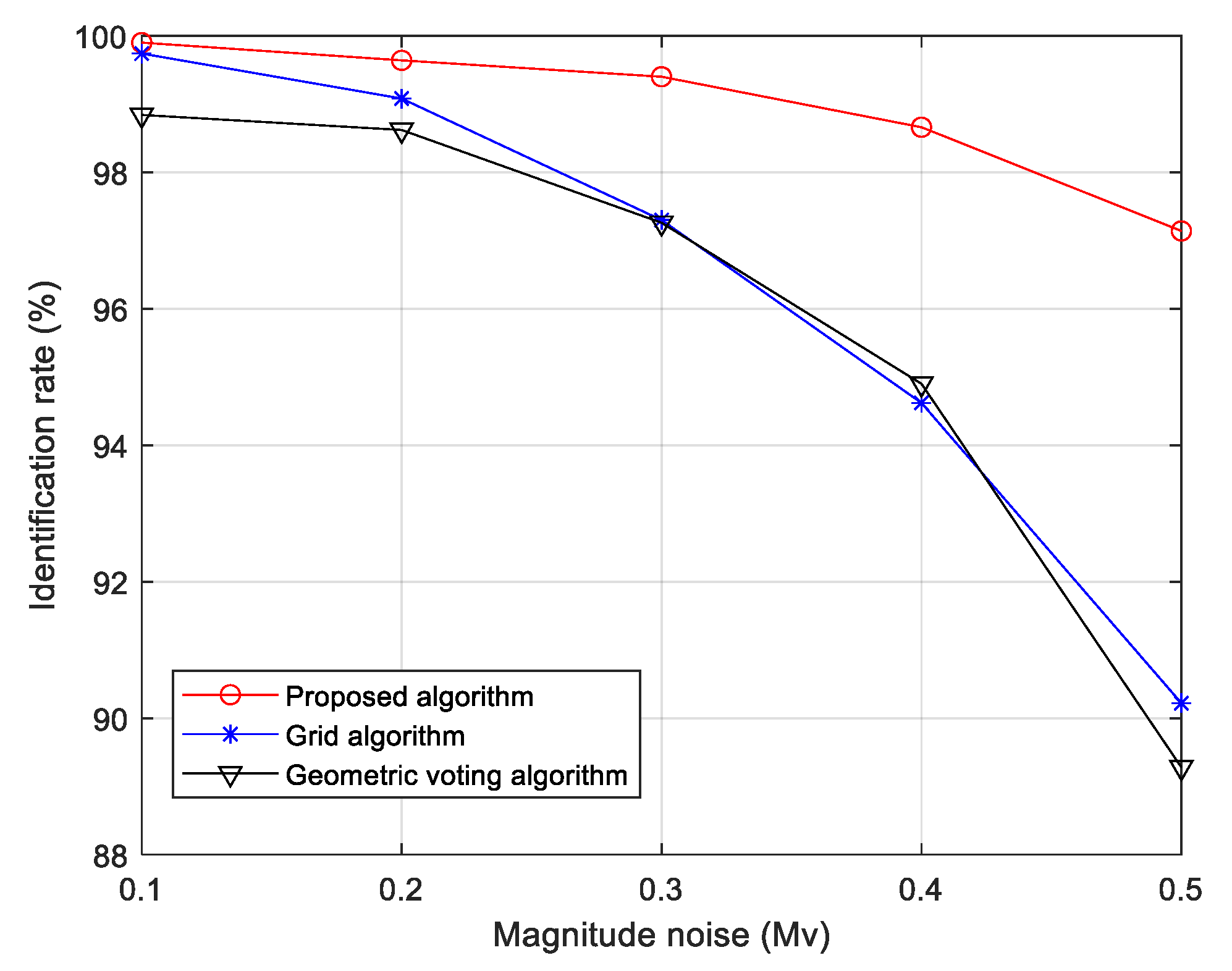
(2). Robustness toward star magnitude noise: Figure 13 illustrates the identification rates of star images for three algorithms when the star magnitude noise increases linearly from 0.1 to 0.5 Mv with a 0.1 Mv step while the position noise is kept at 1.0 pixels.
As shown in Figure 13, the proposed algorithm identification rate drops slightly from 99.9% to 97.14% when the standard deviation of magnitude noise gradually grows from 0.1 to 0.5 Mv. In contrast, the other two reference algorithms obtain a lower identification rate with larger noise; the grid algorithm identification rate decreases to 90.22% while the geometric voting algorithm drops sharply to 89.28% with 0.5 Mv magnitude noise, respectively.
We can see that the magnitude noise deviation increase has less of an effect on the identification performance of the proposed algorithm compared with the two reference algorithms. When the magnitude noise is 0.5 Mv, the identification rate of our algorithm is 6.92% higher than the grid algorithm and 7.86% higher than the geometric voting algorithm. The reasons for this are as follows: some dimmer stars’ appearance and some brighter stars’ disappearance due to magnitude noise cause the wrong closest neighbor star selection and the building of an incorrect grid pattern. For the geometric algorithm, the wrong brighter stars are chosen and receive false votes in the identification process. However, the dimension in the algorithm of the vote unit feature is higher, and it needs fewer correct brighter stars to generate vote units to obtain reliable identification results, so it is more robust to magnitude noise.
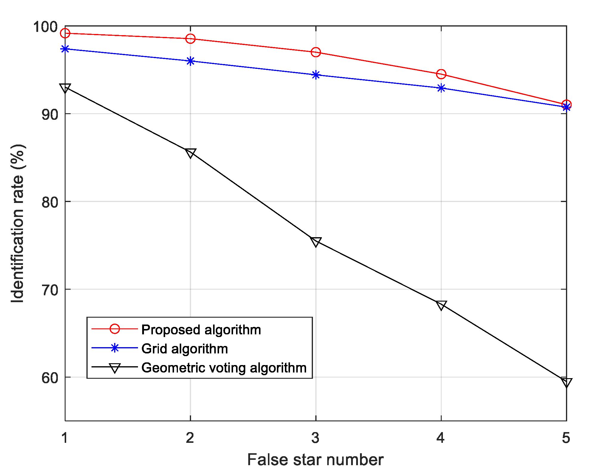
(3). Robustness toward false stars: Figure 14 illustrates the identification rates of star images for the three algorithms as the false star number increases linearly from 0 to 5. In this test, the star position noise and magnitude noise are kept at 1.0 pixels and 0.3 Mv, respectively, while the magnitude value of false stars added to simulated star images varies from 3.5 Mv to 5.5 Mv randomly.
As shown in Figure 14, the proposed algorithm obtains a higher identification rate than reference algorithms as the number of false stars increases from 1 to 5. For our algorithm, the identification rate decreases from 99.16% to 91.02% with false stars increasing, while the identification performance of the geometric voting becomes unsatisfactory when five false stars are added to the image, where it drops significantly to 59.48% and decreases by 33.54% compared with only one false star. The identification rate of the grid algorithm is similar to our algorithm with five false stars, but its identification performance is poorer than our algorithm.
It is obvious that false stars have less influence on the identification performance of the proposed algorithm compared with the other two algorithms. When five false stars are added to the star images, the identification rate of the algorithm is 31.54% higher than the geometric voting algorithm and 0.28% higher than the grid algorithm.
In fact, false stars may be selected as the closest neighbor stars or cause main stars to be identified, which causes the wrong grid pattern to be built, degrading the performance of the algorithm to some extent. Likewise, incorrect vote star pairs are generated when brighter false stars are selected and wrong candidates are obtained in the geometric algorithm. Our algorithm can utilize fewer correct brighter stars to obtain reliable vote results in the identification process, which makes it robust to false stars.
(4). Memory and time performance: Table 2 lists the memory size and running time of the proposed algorithm and the other two reference algorithms, in which memory size is defined as the memory size of the onboard database containing the guide star table and feature table in the algorithm, and run-time is the average time spent identifying a star image with a 1.0-pixel star position noise and 0.3 Mv magnitude noise.
In terms of the run-time performance, our algorithm is 18.36 ms, which is much faster than the grid algorithm (72.71 ms) and geometric voting algorithm (96.86 ms) due to the adopted PCA dimensionality reduction and two-dimension lookup table.
It should be noted that the onboard memory size was very limited in the past, so it is important to pursue a lower database to reduce the required memory cost in algorithm design. However, embedded systems can easily store 5 MB data, and memory size is gradually become a less significant part of the algorithm compared with the identification rate and run time in the star-identification technique. Considering the above factors, it is still acceptable that the proposed algorithm occupies 1.5 MB, which is larger than the reference algorithms.
4. Conclusions
In this paper, a novel star-identification algorithm is proposed to solve the “lost-in-space” problem for star sensors, which utilizes several triangles as a voting unit to obtain the candidates in the initial match, and then a follow-up filter procedure acquires the final results. As the simulation shows, the proposed algorithm is more robust to position noise, magnitude noise, as well as false stars compared with the geometric voting and grid algorithms. Moreover, our algorithm is efficient, and its memory size is acceptable. Therefore, the GMTV algorithm is suitable for future astronautic missions. We will focus on running our algorithm on a hardware system of a star sensor to evaluate its on-orbit performance.
Author Contributions
Funding acquisition, J.Z.; Investigation, X.Y., K.Z., and X.L.; Methodology, X.Y.; Supervision, J.Z.; Validation, X.Y.; Writing—original draft, X.Y.; Writing—review and editing, J.Z. All authors have read and agreed to the published version of the manuscript.
Funding
This work was supported by the National Natural Science Foundation of China (grants no. 61890961) and the Natural Science Basic Research Program of Shaanxi (program no. 2018JM6008).
Institutional Review Board Statement
Not applicable.
Informed Consent Statement
Not applicable.
Data Availability Statement
Not applicable.
Conflicts of Interest
The authors declare no conflict of interest.
References
- Liebe, C.C. Accuracy performance of star trackers-a tutorial. IEEE Trans. Aerosp. Electron. Syst. 2002, 38, 587–599. [Google Scholar] [CrossRef]
- Silani, E.; Lovera, M. Star identification algorithms: Novel approach & comparison study. IEEE Trans. Aerosp. Electron. Syst. 2006, 42, 1275–1288. [Google Scholar]
- Sun, L.; Jiang, J.; Zhang, G.; Wei, X. A discrete HMM-Based feature sequence model approach for star identification. IEEE Sens. 2016, 16, 931–940. [Google Scholar] [CrossRef]
- Mehta, D.S.; Chen, S.; Liang, R.; Low, K.S. A rotation-invariant additive vector sequence based star pattern recognition. IEEE Trans. Aerosp. Electron. Syst. 2018, 55, 689–705. [Google Scholar] [CrossRef]
- Samaan, M.A.; Mortari, D.; Junkins, J.L. Recursive mode star identification algorithms. IEEE Trans. Aerosp. Electron. Syst. 2005, 41, 1246–1254. [Google Scholar] [CrossRef]
- Rijlaarsdam, D.; Yous, H.; Byrne, J.; Oddenino, D.; Furano, G.; Moloney, D. A Survey of Lost-in-Space Star Identification Algorithms Since 2009. Sensors 2020, 20, 2579. [Google Scholar] [CrossRef]
- Padgett, C.; Kreutz-Delgado, K. A grid algorithm for autonomous star identification. IEEE Trans. Aerosp. Electron. Syst. 1997, 33, 202–213. [Google Scholar] [CrossRef]
- Na, M.; Zheng, D.; Jia, P. Modified grid algorithm for noisy all-sky autonomous star identification. IEEE Trans. Aerosp. Electron. Syst. 2009, 45, 516–522. [Google Scholar] [CrossRef]
- Clouse, D.S.; Padgett, C.W. Small field-of-view star identification using Bayesian decision theory. IEEE Trans. Aerosp. Electron. Syst. 2000, 36, 773–783. [Google Scholar] [CrossRef]
- Aghaei, M.; Moghaddam, H.A. Grid star identification improvement using optimization approaches. IEEE Trans. Aerosp. Electron. Syst. 2016, 52, 2080–2090. [Google Scholar] [CrossRef]
- Zhang, G.; Wei, X.; Jiang, J. Full-sky autonomous star identification based on radial and cyclic features of star pattern. Image Vis. Comput. 2008, 26, 891–897. [Google Scholar] [CrossRef]
- Wei, X.; Wen, D.; Song, Z.; Xi, J.; Zhang, W.; Liu, G.; Li, Z. A star identification algorithm based on radial and dynamic cyclic features of star pattern. Adv. Space Res. 2019, 63, 2245–2259. [Google Scholar] [CrossRef]
- Liu, H.; Wei, X.; Jian, L.; Wang, G. A star identification algorithm based on recommended radial pattern. IEEE Sens. 2022, 22, 8030–8040. [Google Scholar] [CrossRef]
- Wei, X.; Zhang, G.; Jiang, J. Star identification algorithm based on log-polar transform. J. Aerosp. Comput. Inf. Commun. 2009, 6, 483–490. [Google Scholar] [CrossRef]
- Jiang, J.; Ji, F.; Yan, J.; Sun, L.; Wei, X. Redundant-coded radial and neighbor star pattern identification algorithm. IEEE Trans. Aerosp. Electron. Syst. 2015, 51, 2811–2822. [Google Scholar] [CrossRef]
- Kim, S.; Cho, M. New star identification algorithm using labelling technique. Acta Astronaut. 2019, 162, 367–372. [Google Scholar] [CrossRef]
- Du, J.; Wei, X.; Jian, L.; Wang, G.; Zang, C. Star identification based on radial triangle mapping Matrix. IEEE Sens. 2022, 22, 8795–8807. [Google Scholar] [CrossRef]
- Liu, L.; Jiang, J.; Zhang, G. Star identification based on spider-web image and hierarchical CNN. IEEE Trans. Aerosp. Electron. Syst. 2019, 56, 3055–3062. [Google Scholar]
- Xu, L.; Jiang, J.; Liu, L. A representation learning-based star identification algorithm. IEEE Access 2019, 7, 91193–92202. [Google Scholar] [CrossRef]
- Yang, S.; Liu, L.; Zhou, J.; Zhao, Y.; Hua, G.; Sun, H.; Zheng, N. Robust and efficient star identification algorithm based on 1D convolutional neural network. IEEE Trans. Aerosp. Electron. Syst. 2022. [Google Scholar] [CrossRef]
- Zhang, G.J.; Wei, X.G.; Jiang, J. Star map identification based on a modified triangle algorithm. Aeronaut. Astronaut. Sin. 2006, 27, 1150–1154. [Google Scholar]
- Fang, J.; Quan, W.; Meng, X. All-sky autonomous star map identification algorithm based on Delaunay triangulation cutting algorithm. J B Univ Aeronaut Astronaut 2005, 31, 311–315. [Google Scholar]
- Sun, L.; Zhou, Y. MVDT-SI: A Multi-View Double-Triangle Algorithm for Star Identification. Sensors 2020, 20, 3027. [Google Scholar] [CrossRef] [PubMed]
- Mortari, D.; Samaan, M.A.; Bruccoleri, C.; Junkins, J.L. The pyramid star identification technique. Navigation 2004, 51, 171–183. [Google Scholar] [CrossRef]
- Kolomenkin, M.; Pollak, S.; Shimshoni, I.; Lindenbaum, M. Geometric voting algorithm for star trackers. IEEE Trans. Aerosp. Electron. Syst. 2008, 44, 441–456. [Google Scholar] [CrossRef]
- Quine, B.M.; Durrant-Whyte, H.F. A fast autonomous star-acquisition algorithm for spacecraft. Control. Eng. Pract. 1996, 4, 1735–1740. [Google Scholar] [CrossRef]
- Wang, Z.; Quan, W. An all-sky autonomous star map identification algorithm. IEEE Trans. Aerosp. Electron. Syst. 2004, 19, 10–14. [Google Scholar] [CrossRef]
- Wang, G.; Jian, L.; Wei, X. Star identification based on hash map. IEEE Sens. 2017, 18, 1591–1599. [Google Scholar] [CrossRef]
- Zhao, Y.; Wei, X.; Jian, L.; Wang, G. Star identification algorithm based on K–L transformation and star walk formation. IEEE Sens. 2016, 16, 5202–5210. [Google Scholar] [CrossRef]
Figure 1.
Triangle unit built.

Figure 2.
Database structure.

Figure 3.
Feature unit storing process in the database.

Figure 4.
The process of the algorithm.

Figure 5.
Fuzzy search strategy.

Figure 6.
Vote process in the initial match step.

Figure 7.
A connection matrix.

Figure 8.
Searching initial largest cluster.

Figure 9.
Filtering initial largest cluster elements.

Figure 10.
Extend the core cluster.

Figure 11.
Identification rate versus positional noise with different discretized unit.

Figure 12.
Identification rate versus positional noise.

Figure 13.
Identification rate versus magnitude noise.

Figure 14.
Identification rate versus false star.


Table 1.
Key parameters of sensor star.
| Field of View | 25° × 25° |
|---|---|
| Resolution | 1024 × 1024 |
| Pixel size | 15 μm |
| Focal Length | 34.64 mm |
| Minimum Sensitivity | 5.5 Mv |
Table 2.
Time and memory size.
| Algorithm | Our Method | Grid | Geometric Voting |
|---|---|---|---|
| Run time | 18.36 ms | 72.71 ms | 96.86 ms |
| Memory size | 1.5 MB | 0.5 MB | 0.6 MB |
Publisher’s Note: MDPI stays neutral with regard to jurisdictional claims in published maps and institutional affiliations. |
© 2022 by the authors. Licensee MDPI, Basel, Switzerland. This article is an open access article distributed under the terms and conditions of the Creative Commons Attribution (CC BY) license (https://creativecommons.org/licenses/by/4.0/).
Share and Cite
MDPI and ACS Style
Yuan, X.; Zhu, J.; Zhu, K.; Li, X. A Star-Identification Algorithm Based on Global Multi-Triangle Voting. Appl. Sci. 2022, 12, 9993. https://doi.org/10.3390/app12199993
AMA Style
Yuan X, Zhu J, Zhu K, Li X. A Star-Identification Algorithm Based on Global Multi-Triangle Voting. Applied Sciences. 2022; 12(19):9993. https://doi.org/10.3390/app12199993
Chicago/Turabian StyleYuan, Xiaobin, Jingping Zhu, Kaijian Zhu, and Xiaobin Li. 2022. "A Star-Identification Algorithm Based on Global Multi-Triangle Voting" Applied Sciences 12, no. 19: 9993. https://doi.org/10.3390/app12199993
Note that from the first issue of 2016, this journal uses article numbers instead of page numbers. See further details here.