Article

CD_HIEFNet: Cloud Detection Network Using Haze Optimized Transformation Index and Edge Feature for Optical Remote Sensing Imagery

1
Aerospace Information Research Institute, Chinese Academy of Sciences, Beijing 100094, China
2
School of Electronic, Electrical and Communication Engineering, University of Chinese Academy of Sciences, Beijing 100049, China
*
Author to whom correspondence should be addressed.
Remote Sens. 2022, 14(15), 3701; https://doi.org/10.3390/rs14153701
Submission received: 1 July 2022 / Revised: 28 July 2022 / Accepted: 30 July 2022 / Published: 2 August 2022

Abstract

:
Clouds in optical remote sensing images are an unavoidable existence that greatly affect the utilization of these images. Therefore, accurate and effective cloud detection is an indispensable step in image preprocessing. To date, most researchers have tried to use deep-learning methods for cloud detection. However, these studies generally use computer vision technology to improve the performances of the models, without considering the unique spectral feature information in remote sensing images. Moreover, due to the complex and changeable shapes of clouds, accurate cloud-edge detection is also a difficult problem. In order to solve these problems, we propose a deep-learning cloud detection network that uses the haze-optimized transformation (HOT) index and the edge feature extraction module for optical remote sensing images (CD_HIEFNet). In our model, the HOT index feature image is used to add the unique spectral feature information from clouds into the network for accurate detection, and the edge feature extraction (EFE) module is employed to refine cloud edges. In addition, we use ConvNeXt as the backbone network, and we improved the decoder to enhance the details of the detection results. We validated CD_HIEFNet using the Landsat-8 (L8) Biome dataset and compared it with the Fmask, FCN8s, U-Net, SegNet, DeepLabv3+ and CloudNet methods. The experimental results showed that our model has excellent performance, even in complex cloud scenarios. Moreover, according to the extended experimental results for the other L8 dataset and the Gaofen-1 data, CD_HIEFNet has strong performance in terms of robustness and generalization, thus helping to provide new ideas for cloud detection-related work.

Graphical Abstract

1. Introduction

With the rapid development of remote sensing technology, the field of satellite remote sensing has entered the era of Big Data [1,2,3]. Remote sensing is now widely used in environmental protection, land resource surveys, disaster monitoring and other fields [4,5,6]. According to the long-term observations of the International Satellite Cloud Climatology Project (ISCCP), more than 60% of the Earth’s surface is regularly covered by clouds [7]. Therefore, optical remote sensing images are easily disturbed by the atmosphere and clouds, and many images are occluded by clouds. Due to cloud occlusion, the information for ground objects can be attenuated or even lost and the texture of and spectral information from the images may be changed at the same time, which adversely affects the subsequent production of images and seriously reduces the utilization rate of remote sensing images [8,9]. Furthermore, studying the distribution of clouds is helpful for investigations of climate change trends, and it is also significant for the assessment of the global surface radiation budget [10,11,12]. Therefore, cloud detection is key to subsequent image identification, classification and interpretation, and it is the premise that guarantees the production of seamless spatiotemporal remote sensing products [13]. Moreover, effective cloud detection is also an important step in cloud removal [14,15]. Cloud detection can also be used to eliminate images with excessive cloud coverage in order to reduce the burden on data storage and improve product production efficiency. Efficient and accurate cloud detection in remote sensing images has also become a hot issue in the field of remote sensing.
Cloud detection is a semantic segmentation process for pixel-level image classification based on actual semantic information, and it is also a binary classification problem based around distinguishing cloud and non-cloud areas. In the past few decades, much research has been undertaken on cloud detection using different methods. These methods include the spectral threshold method, the texture analysis method and the machine-learning method [16,17,18]. The spectral threshold method mainly relies on the spectral characteristics of clouds and involves designing different combinations of various bands for detection. This method is widely used with MODIS data and Landsat data. Jedlovec [19] used 19 channels of MODIS data and terrain data for cloud detection in the popular MODIS Cloud Mask cloud detection method. Irish et al. [20] proposed an automatic cloud cover assessment (ACCA) algorithm for Landsat 7 images that uses spectral characteristics to perform the first scan and then the radiance and temperature characteristics to perform the second scan and obtain cloud detection results. Subsequently, Zhu et al. [21] proposed the function of mask (Fmask) algorithm to extract clouds and cloud shadows with high accuracy in Landsat data. In recent years, in view of the variability in remote sensing images, a dynamic threshold has been developed as part of the spectral threshold method to obtain more accurate detection results [22,23]. However, most of these methods require the use of many bands, and threshold determination is complicated. Moreover, most of them are designed for specific sensors and cannot be generalized to other sensors, so it is difficult to for these methods to be universal.
With the continuous improvement in the spatial resolution of remote sensing images, the texture features of clouds and ground objects are becoming more obvious in images. Therefore, cloud detection methods based on texture analysis have also attracted the attention of many scholars. The most widely used texture features of clouds are the gray level co-occurrence matrix (GLCM), the fractal dimension and the boundary feature [17]. Kittler and Pairman [24] used the GLCM to construct the feature space of clouds, and this method was able to effectively distinguish cloud and non-cloud areas. However, the method still misjudged thin cloud areas. Cao et al. [25] constructed a two-dimensional feature space with the fractal dimension and GLCM and used a plane classifier to distinguish clouds and ground objects in order to achieve fast and accurate cloud detection. Wang et al. [26] adopted four edge features for cloud recognition, which reduced the misjudgment rate for some mountainous and snowy areas, but it was difficult to distinguish clouds in completely white images of snow. Although this method has improved accuracy compared to the threshold method, the extraction of texture features entails significant computation costs and it still does not address the problem of threshold determination.
Cloud detection methods based on machine learning can be divided into traditional machine-learning methods and deep-learning methods. Although traditional machine-learning methods, such as clustering [27], artificial neural networks [28], support vector machines [29] and random forest algorithms [30], can solve the threshold problem and improve cloud detection accuracy, they require manual selection of features and cannot complete end-to-end learning. In recent years, deep learning has been developing with unprecedented speed. Compared to traditional algorithms, deep learning has strong learning portability and can extract complex nonlinear features. As a typical deep-learning method, convolutional neural networks (CNNs) are widely used in natural language processing, image classification and other fields. Since fully convolutional networks (FCNs) [31] were proposed in 2014, semantic segmentation networks have become the dominant method for image segmentation, including cloud detection. Mohajerani et al. [32] applied an FCN for cloud detection in Landsat data and obtained an accuracy of 88%, but the types of underlying surfaces studied in this method were limited, resulting in poor generalization. Lu et al. [33] used SegNet with multi-scale filters to reduce the probability of identifying other objects as clouds, but the ability to distinguish clouds and snow still required improvement. Peng et al. [34] found that DeepLabv3+ has high accuracy and stability for cloud recognition because of the atrous spatial pyramid pooling (ASPP) module, which makes it possible to obtain advanced features of different scales, but it has the shortcomings including spatial information loss and overly smooth boundaries.
Researchers have also explored networks specifically designed for cloud detection. Zhan et al. [35] added low-level spatial information to a network to improve cloud discrimination. Mohajerani et al. [36] redesigned a fully convolution network to combine global and local features for cloud detection, naming the new method CloudNet. In addition, some studies have also found that fusing CNNs with handcrafted features can improve the performance of cloud detection networks. Zhang et al. [37] added Gabor-filtering feature extraction and channel attention modules to U-Net so that the network could learn rich details and the accuracy of cloud detection could be improved. Guo et al. [38] fused mean, Gabor and Laplacian features to make the network more advanced and accurate. The deep-learning method can achieve end-to-end learning and has high accuracy and universality, but the existing semantic segmentation networks still need improvements for cloud detection. A general segmentation network is mainly divided into two parts: the encoder and decoder. In the encoder part, in order to obtain the global information for image and reduce the amount of calculation, the network needs multiple downsampling operations, but the downsampling process leads to spatial information loss, resulting in inaccurate boundary definitions and affecting the accuracy of cloud detection. Moreover, most cloud detection networks are based on the application of computer vision to the original network. Although the related texture features are integrated, they do not incorporate the unique band feature information from remote sensing images, which means that such networks have certain limitations for cloud detection.
Researchers have also come to understand the difference between remote sensing images and natural images and have studied semantic segmentation networks based on the particularity of remote sensing images. Su et al. [39] used the normalized difference water index (NDWI) together with original images as the input for the DeepLabv3+ network in order to investigate water extraction and found that using the NDWI images as input resulted in the network paying much more attention to water extraction. Therefore, inspired by this work, and in view of the lack of attention paid to the multi-band rate characteristics of remote sensing images in existing cloud detection networks and the difficulty of detecting cloud edge details, this paper proposes a new cloud detection network using the haze-optimized transformation (HOT) index and edge feature extraction based on the most common red, blue, green and near-infrared bands (CD_HIEFNet). The main contributions of this paper are as follows:
  • We used the HOT index image and the multispectral (MS) image together as the input of the network, which added the spectral characteristics of the clouds and enabled the network to distinguish difficult regions that are easily confused with clouds, so that the network could distinguish regions that are easily confused with clouds;
  • We deployed an edge feature detection (EFE) module to enhance the extraction of cloud boundary details in the network. This made the network fit the cloud boundary well and allowed it to detect various cloud types;
  • In our structure, we adopted ConvNeXt [40] as the backbone network. In the decoder stage, we used a structure to fuse shallow and deep features from bottom to top to compensate for the loss of edge and local information, which made it possible to recover boundary information effectively and obtain accurate results;
  • CD_HIEFNet has great cloud detection performance for Landsat-8 (L8) Biome datasets. Moreover, the extended experiments showed that CD_HIEFNet had good generalization performance, which is important in practical applications.
The remainder of this paper is arranged as follows. In Section 2, the theoretical methodology for and structural design of CD_HIEFNet are described. In Section 3, the data, the experiments and the corresponding experimental results used to verify the superior performance of CD_HIEFNet are described. Section 4 presents the conclusion.

2. Methodology

Current semantic segmentation networks generally employ an encoder–decoder structure. The encoder usually uses image classification networks, such as VGGNet [41] and ResNet [42], to extract the image features through multi-layer convolution. Many improved modules have also been proposed for semantic segmentation networks, such as the ASPP module [43], to fuse multi-scale spatial information. The decoder stage projects the discriminative features learned by the encoder semantically into the pixel space to obtain a dense classification. Existing decoding mechanisms include the skipping connection [44] and inverse pooling upsampling [45]. A good semantic segmentation network needs not only discriminative abilities at the pixel level but also the ability to incorporate the discriminative features learned by the encoder at different stages.
Our proposed CD_HIEFNet network is also based on the encoder–decoder structure, and the overall framework of the network is shown in Figure 1. As shown in the figure, the initial input of our network consists of two parts: (1) red, green, blue and near-infrared band remote sensing images; (2) HOT index spectral feature images. The encoder uses ConvNeXt with good accuracy and scalability as the backbone network. In addition, the EFE module was added to this part to enhance the attention paid to edge information, as well as the ASPP module to fuse multi-scale and global context information. The backbone network, the HOT index and the EFE module are described in detail in Section 2.1, Section 2.2 and Section 2.3.
At the decoder stage, the fusion of feature information from different stages and different scales can improve the final segmentation results. The feature pyramid network (FPN) [46] uses a pyramid architecture with lateral connections based on the inherent multi-scale pyramid hierarchy of the encoder, enabling the network to obtain precise semantic features and feature locations. We borrowed the pyramid structure of the FPN. In accordance with the downsampled pyramid structure of the classification network, we started by upsampling the feature map with the lowest spatial resolution but the strongest semantic spatial resolution by a factor of 2 (using bilinear interpolation upsampling) and then used element-wise addition to merge the upsampled map with the corresponding level map (a 1 × 1 convolutional layer was applied to the corresponding level map to change the channel dimensions and ensure an equal number of channels). This process was iterated until the result was generated at the top level of the classification network pyramid structure. After this operation, the output results of each layer had complementary relationships, and convolution fusion could be used to obtain accurate segmentation results. In addition, similar to the holistically nested edge network (HDE) [47], we performed 3 × 3 convolution on the abovementioned results from each layer and generated three side output saliency probability maps: Side 1, Side 2 and Side 3. Then, we upsampled them to the original image size and concatenated them, performing 1 × 1 convolution to generate the final saliency probability map.

2.1. Backbone Network

The backbone network plays a crucial role in improving both the efficiency and accuracy of segmentation. Focusing on accuracy, efficiency and scalability, CNNs have launched many representative networks [40], such as VGGNet, ResNet, MobileNet [48] and EfficientNet [49]. However, vision transformers (ViTs) [50] have been widely used in image classification since their development, and they have advantages such as scalable behavior and multi-head attention. On the other hand, in computer vision downstream tasks such as object detection and semantic segmentation, vanilla ViTs face difficulties due to the increased complexity of the attention mechanism. Swin Transformers [51] solve the problem by using a hierarchical structure similar to that used in CNNs and local attention, making these transformers viable as a general visual backbone network; however, it also shows that CNNs are still needed in image segmentation tasks. Therefore, ConvNeXt networks have been built with standard convolutional modules, but they borrow the structure and training mode from transformers to obtain high accuracy and scalability comparable to transformers in the networks [40].
Cloud detection is usually applied in the context of large-scale remote sensing image data, so efficiency is also an issue to be considered. Therefore, we selected the improved version of ConvNeXt-T with the smallest amount of parameters as the backbone network. ConvNeXt-T is composed of a stack of four stages, as shown in Table 1. Stage 1 uses a 4 × 4 convolution with a stride of 4 and layer normalization (LN) to directly downsample the image to one quarter of the input image size and then goes through three ConvNeXt blocks (Figure 2a). Stage 2 consists of a downsampling block (Figure 2b) and three ConvNeXt blocks. Stage 3 is also composed of a downsampling block, as well as nine ConvNeXt blocks. Stage 4 is different from the original ConvNeXt network structure. Chen et al. [52] found that too much downsampling can make the spatial resolution overly low, making it difficult to recover spatial information. However if no downsampling is performed, too much memory space will be used and the complexity will be increased. The authors proved that the best downsampling step to maintain efficiency and accuracy is 1/16. Therefore, in the last stage, we used ordinary convolution with a kernel size of 3 × 3 instead of downsampling, and then three ConvNeXt blocks. At the same time, the dilation rate of the convolution was changed to 2 to ensure that the network continued to acquire deep features without any reduction in the receptive field.

2.2. HOT Index Extraction

Numerous spectral characteristic indexes are available for cloud detection using the spectral threshold method, but many of them use the mid-infrared and thermal infrared bands, which are not universally applicable. Most remote sensing images only contain red, green, blue and near-infrared bands. The HOT index only needs red and blue bands, which have strong universality and high computational efficiency. Therefore, we used the HOT index as the cloud spectral feature index in this study, and the HOT index feature image and the original MS image were used as the input of the network.
The HOT index was originally designed to detect clouds and haze in Landsat 7 data [53], and it has been modified by Zhu et al. [21]. It is currently widely used in thin-cloud detection, cloud removal and fog removal. The design principle of the HOT index is that the reflectivities of cloud and non-cloud areas in the blue and red bands have certain differences. Generally speaking, the HOT index of a cloud is relatively large, so the cloud area can be effectively extracted. The formula is as follows [21]:
HOT = B     0.5   ×   R     0.08
where B is the top of atmosphere (TOA) reflectance of the blue band and R is the TOA reflectance of the red band.

2.3. Edge Feature Extraction Module

In the process of cloud detection, the cloud body is easy to detect due to it being quite different from other ground objects. However, the cloud boundary can easily be mixed with the surrounding pixel information. In addition, cloud boundaries are complex and diverse, making them difficult to accurately detect. In fact, accurate detection of boundaries can greatly improve the accuracy of cloud detection. Therefore, inspired by the Gabor feature extraction module of Zhang et al. [37], we employed the EFE module to enhance the edge detection ability of our network. We adopted the commonly used edge detection operator known as the Sobel operator for edge feature extraction.
The Sobel operator uses two 3 × 3 kernels convolved with the image to calculate approximations of the derivatives—one for horizontal changes and the other for vertical changes. The calculations are shown in Equation (2):
G x = [ f ( x + 1 , y 1 ) + 2 f ( x + 1 , y ) + f ( x + 1 , y + 1 ) ] [ f ( x 1 , y 1 ) + 2 f ( x 1 , y ) + f ( x + 1 , y + 1 ) ] G y = [ f ( x 1 , y 1 ) + 2 f ( x , y 1 ) + f ( x + 1 , y 1 ) ] [ f ( x 1 , y + 1 ) + 2 f ( x , y + 1 ) + f ( x + 1 , y + 1 ) ]
where f ( x , y ) is the gray value at ( x , y ) in the image, and G x ,   G y are approximations of the gray partial derivatives in the horizontal and vertical directions, respectively, which result from the plane convolution of the original image in both directions.
Then, for each point in the image, the final gradient can be obtained from the square root of the square sum of the gradients G x and G y . In practical applications, in order to improve efficiency, an approximation calculation without the square root is used. The calculation formula is shown in Equation (3):
G = | G x | + | G y |
where G is the final gradient.
There is a large amount of edge detail information in low-level features. Considering the computational efficiency of the network and in order to obtain as much edge information as possible, we only added the EFE module to the initial input image. As shown in Figure 3, the EFE module first performs a 3 × 3 convolution to the input image. It can add affluent channels and extract low-level features, which is beneficial to the Sobel operator to obtain fine edge details. After using the Sobel operator, it is possible to automatically learn the difference between the image after edge extraction and the image without edge extraction through the subtraction and convolution operations. Then, the learned difference information is added to the image without edge extraction to obtain an edge enhancement effect, which helps the network accurately locate and restore edge details. Moreover, in this module, so as to speed up the training convergence of the network and reduce overfitting, batch normalization (BN), which is often employed for normalization in networks, is used after each convolution.

2.4. Focal Loss

Sample imbalance is a common phenomenon in the application of deep learning to vision tasks. In the process of cloud detection, this imbalance may even be obvious: in some images, large clouds appear continuously, while other images have very small proportions of clouds. This situation makes it difficult for networks to learn small-scale categories, resulting in poor model accuracy. The key to alleviating this problem is to increase the weight of small-scale categories and thus ensure the balance between different categories. However, the method for manually setting the weight requires many attempts, and the degree of automation and universality is poor. Therefore, we used focal loss [54] as the loss function in this study, as it can automatically adjust the weight according to the difficulty learning the sample to ensure the network works well for cloud detection.
Focal loss is a loss function proposed for target detection when the foreground and background are unbalanced. It makes the network focus on learning difficult samples by reshaping the standard cross-entropy. Equation (4) is the standard cross-entropy formula [55], and Equation (5) is the formula for focal loss:
C E ( p t ) = log ( p t )
FL ( p t ) = ( 1 p t ) γ log ( p t )
where p t is the model prediction probability, and γ is the set parameter; we set it to 2 in accordance with the best experimental result obtained in the original paper [54]. When p t is small, this means that the sample has been misclassified and the corresponding ( 1 p t ) γ increases, so that the network will not ignore learning the misclassified sample. Conversely, when p t approaches 1, this indicates that the sample has been classified well. The ( 1 p t ) γ then changes to 0 and the sample is down-weighted.

3. Results and Discussion

3.1. Dataset Processing

Model training for deep-learning networks requires large and high-quality datasets. The L8 global cloud cover assessment validation dataset “L8 Biome Cloud Validation Masks” (L8 Biome) [56] is an internationally recognized cloud detection dataset. The L8 Biome dataset is used in most cloud detection studies due to its rich selection of surface types, the variety of which is beneficial for the performance of networks. We also chose the L8 Biome dataset as our source for model training and validation. We further selected the L8 Spatial Procedures for Automated Removal of Cloud and Shadow (SPARCS) dataset [57] and Gaofen-1 (GF-1) data to verify the generalization ability of the network model.

3.1.1. Datasets

  • The L8 Biome dataset: This dataset includes 96 L8 images sampled from all over the world with sizes of 8000 × 8000 (30 m resolution) and manually generated cloud masks. The dataset has eight types of scene—urban, forest, shrubland, grass, snow, barren, wetlands and water—and each scene type contains 12 images. In order to ensure data heterogeneity and diversity, images are selected with different paths/rows and cloud patterns;
  • The SPARCS dataset: This consists of 80 sub-images of L8 images, and the size is 1000 × 1000 (30 m resolution). The purpose of the dataset was to select 12 additional scenarios to use in evaluating the classifier and to reduce the risk of overfitting. Therefore, it was used as the extended experimental data in this study;
  • GF-1 data: The GF-1 satellite is equipped with a panchromatic/multispectral (PMS) camera. The PMS camera can acquire panchromatic images with a resolution of 2 m and MS images with a resolution of 8 m (four bands—blue, green, red and near-infrared), with sizes of approximately 5000 × 5000. The spectral range and the spatial resolution of GF-1 are different from those of L8. Therefore, we also used the MS images as extended experimental data to further verify the scalability of the network.

3.1.2. Pre-Processing

The original cloud masks of the L8 Biome Dataset are divided into four categories: cloud shadow, clear, thin cloud and cloud. In this study, the main purpose was to detect clouds, so we combined the cloud masks into two categories: cloud and non-cloud. Since the calculation of the HOT index requires the TOA reflectance, we first performed radiometric calibration to convert the DN value to the TOA reflectance. Next, we selected the red, green, blue and near-infrared bands from the original image to synthesize the four-band images, and then we calculated the HOT index feature image. We also performed the same radiometric calibration and feature calculation process for the SPARCS dataset and the GF-1 data.
As the L8 image size was too large and our hardware processing capabilities for the experiment were limited, we cut the image into non-overlapping sub-images with sizes of 512 × 512 and obtained 18,466 sub-images. Then, we randomly divided the sub-images into the training set, the validation set and the test set accodring to the ratio of 6:1:3. The training set was used to train the network model, the validation set was used to adjust the model parameters during the training process and the test set was only used to evaluate the model performance and did not participate in the training process. The SPARCS dataset and GF-1 data were also cropped to the size of 512 × 512.
In addition, in order to ensure the network had strong generalization and robustness, we used data augmentation to enhance the number and complexity of training samples. We used a data augmentation strategy with random flips and random rotations. Figure 4 shows the original image and the data augmentation results. Finally, our dataset contained 33,237 training images, 1847 validation images and 5540 testing images.

3.2. Experiment Settings

3.2.1. Implementation Details

We implemented our network in the open source Pytorch [58] framework and executed it on a 64-bit Ubuntu 18.04 computer with two GeForce RTX 3090 GPU 24 GB cards. We used the stochastic gradient descent (SGD) optimizer with an initial learning rate of 0.001, momentum of 0.9 and weight decay of 0.0005. The cosine annealing learning rate strategy [59], which uses a slow-acceleration, slow-decline mode, reduces the learning rate through the cosine function. It has a good effect on network performance. Therefore, we used the cosine annealing learning rate strategy as the learning rate decay method, with a minimum learning rate of 1 × 10⁻⁸. When training the model, we set the batch size to 16 and carried out 40,000 iterations. To prevent overfitting, the drop path was added to the ConvNeXt block. The specific steps of our cloud detection model training and verification are shown in Algorithm 1.
Algorithm 1. Cloud detection model training and verification
Input: D a t a t r a i n ,   D a t a v a l , D a t a t e s t are the data for model training, validation and testing, respectively; S P A R C S i m g and G F i m g are the images for the extended experiment; i t e r is the number of iterations; m a x i t e r is the maximum number of iterations; n e t is the initial network.
Output: model prediction results: D a t a p r e d ,   S P A R C S p r e d ,   G F p r e d ; model: n e t i t e r ,   m o d e l i t e r ,   m o d e l b e s t ; evaluation index: O A v a l ,   O A t e s t ,   P R t e s t ,   R R t e s t ,   F 1 t e s t ,   m I O U t e s t .
1: while i t e r < m a x i t e r do
2: n e t D a t a t r a i n
3: n e t i t e r update net parameters
4: if i t e r % 200 == 0 then
5: O A v a l n e t i t e r evaluate D a t a v a l
6: m o d e l i t e r save the n e t i t e r
7: end if
8: end while
9: m o d e l b e s t choose the best model in m o d e l i t e r by O A v a l
10: D a t a p r e d m o d e l b e s t predict D a t a t e s t
11: O A t e s t ,   P R t e s t ,   R R t e s t ,   F 1 t e s t ,   m I O U t e s t compare D a t a p r e d with D a t a t e s t
12: S P A R C S p r e d ,   G F p r e d m o d e l b e s t perform cloud detection for S P A R C S i m g and G F i m g

3.2.2. Evaluation Metrics

In order to quantitatively evaluate the performance of our network, we used the overall accuracy (OA), precision ratio (PR), recall ratio (RR), F1 score and the mean intersection of union (mIOU) as evaluation metrics. Their calculation formulae are expressed as follows:
OA = T P + T N T P + F P + T N + F N
PR = T P T P + F P
RR = T P T P + F N
F 1   score = 2 PR * RR PR + PR
mIOU = 1 N + 1 i = 0 N T P T P + F N + F P
where T P denotes the number of cloud samples that are correctly predicted as cloud samples, T N denotes the number of non-cloud samples that are correctly predicted as non-cloud samples, F P denotes the number of non-cloud samples that are wrongly predicted as cloud samples and F N denotes the number of cloud samples that are wrongly predicted as non-cloud samples.

3.3. Ablation Experiments

To verify the effectiveness of our proposed ideas, we analyzed the network prediction accuracy of the different modules in our model under the ConvNeXt backbone network. For a fair comparison, all cases were trained, validated and tested on the same dataset with the same hyperparameters. The results are shown in Table 2. Representative cloud detection comparison results are also shown in Figure 5.
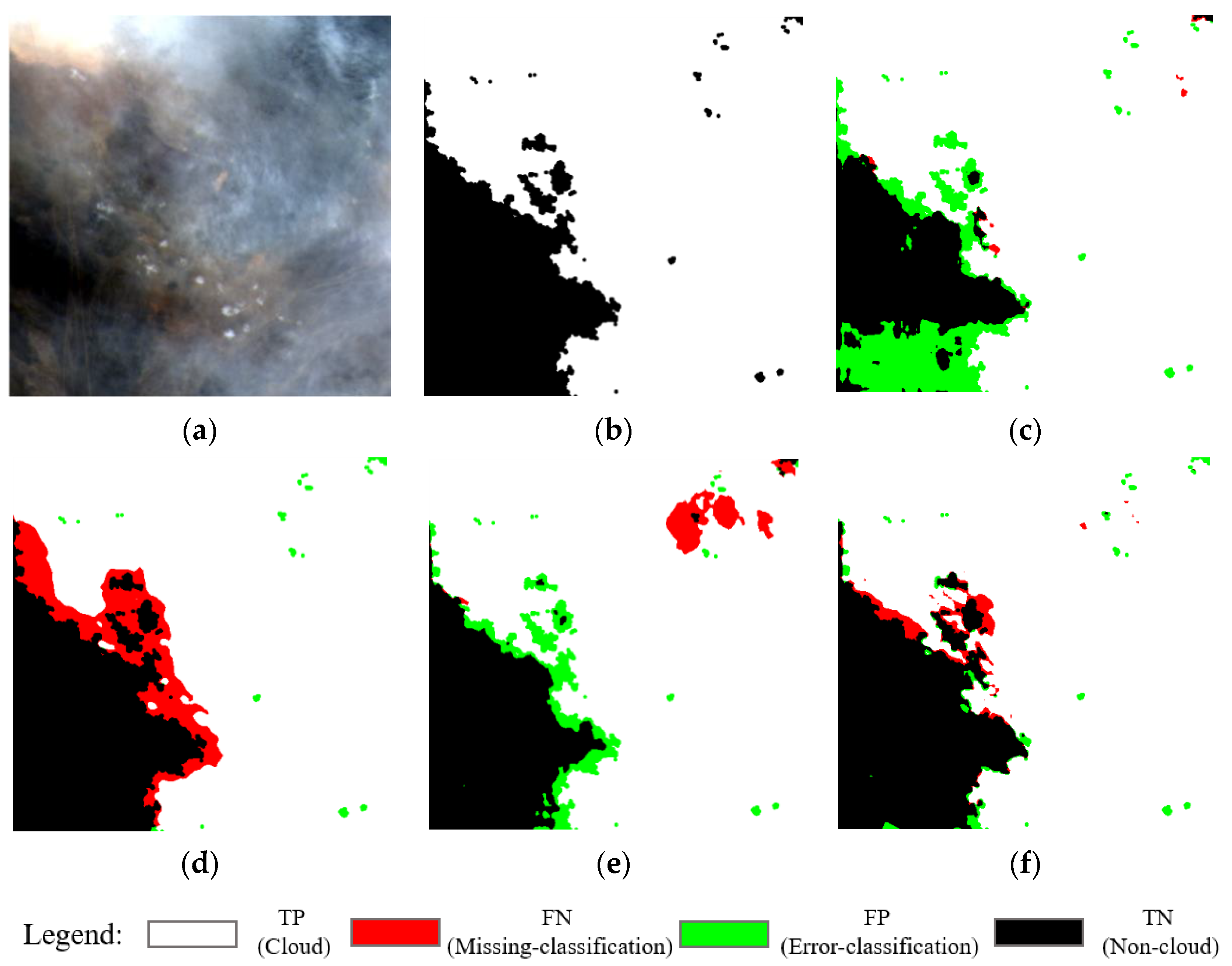
  • Effectiveness of the HOT index: Spectral feature information is helpful in extracting clouds. In Table 2, it can be seen that, compared with the network without the HOT index, most of the evaluation indicators for the network with the HOT index were improved. The greatly improved PR shows that the addition of the HOT index spectral feature information was indeed beneficial for cloud detection. In Figure 5a–c, we can also see that the addition of the HOT index added the spectral feature information of the cloud to the network, which made it possible to effectively eliminate some confusing non-cloud pixels around thin clouds to improve accuracy;
  • Effectiveness of the EFE module: Edge information plays a critical role in cloud detection. In Table 2, it is can be seen that the performance improvement resulting from the EFE module was much greater than that of the HOT index. The EFE module increased the OA value from 95.52% to 96.28%, the PR from 93.87% to 95.54%, the RR from 94.76% to 95.08%, the F1 score from 94.31% to 95.55% and the mIOU from 91.06% to 92.53%. In Figure 5c, it can be seen that the addition of the EFE module made the detection results more accurate, and the boundary fitting of the cloud was also strengthened. However, there were some pixels that were mistaken for non-cloud areas due to weak boundaries between thick and thin clouds;
  • Effectiveness of the fusion of the HOT index and the EFE module: As shown in Table 2, the best performance for the network resulted from the fusion of the HOT index and the EFE modules, with which the OA increased by 1.0%, the PR increased by 1.7%, the RR increased by 0.8%, the F1 score increased by 1.2% and the mIOU increased by 1.8%. It can be seen in Figure 5f that the models that fused the two modules exhibited more accurate cloud detection results and finer edges. Only adding the EFE module caused a weak boundary error (see Figure 5e), but the spectral feature information added by the HOT index alleviated this situation. Moreover, the edge information extracted by the EFE module enabled some pixels with similar spectral features to be distinguished and the performance improved.

3.4. Comparative Experiments

To demonstrate the effectiveness and accuracy of the network, we compared the proposed CD_HIEFNet network with classical methods, including Fmask [21], FCN8s (the prediction result is upsampled by a factor of 8) [31], U-Net [44], SegNet [45], DeepLabv3+ (the backbone network is Xception) [43] and CloudNet [36]. They were evaluated using the same dataset with the same training parameter settings. The quantitative results are shown in Table 3. Furthermore, in order to show the performance of the network with various surface types, we also selected representative cloud detection results for nine surface types for visualization and qualitative analysis: barren, forest, grass, shrubland, snow, urban, building and wetlands, as shown in Figure 6, Figure 7, Figure 8, Figure 9, Figure 10, Figure 11, Figure 12, Figure 13 and Figure 14, respectively.
As can be seen from Table 3, deep-learning methods had obvious advantages over Fmask. Fmask combines multi-band spectral information for cloud detection, which can have a certain detection effect, but simple decision-making based on thresholds still resulted in poor detection results. Due to the ability to fit complex features using deep learning, other networks all had high accuracy for cloud detection. For FCN8s, VGG16 net was used for feature extraction, and the deep features and shallow features were well-fused at the decoder stage, so it showed good detection results. In the evaluation results for U-Net, SegNet and CloudNet, the RRs were higher than the PRs, but DeepLabv3+ had a higher PR than RR. The reason for this is that U-Net and SegNet use skip connections and inverse pooling upsampling mechanisms, respectively, at the decoder stage to closely combine deep and shallow features, allowing them to better restore pixel details. CloudNet uses shortcut connections in each block to capture the global and local features and present details. DeepLabv3+, on the other hand, simply fuses with one of the shallow features to restore the detailed information, resulting in lower recall. However, at the encoder stage, DeepLabv3+ introduces the ASPP module to obtain multi-scale information, and this module can acquire more global and accurate semantic features, so the precision of the cloud detection results was greatly improved compared to other networks. Our proposed network CD_HIEFNet performed the best in the detection results among all the networks. It not only had high accuracy but also maintained a low missed-detection rate and a high recall rate. The results benefited from our designed encoder and decoder. We selected ConvNeXt as the backbone network, added the HOT index image and introduced the ASPP module to obtain more accurate semantic features. The improved decoder enabled our network to combine the deep and shallow features closely and locate the boundary accurately and the EFE module enhanced the edge information, resulting in the network achieving optimal detection of edge and detail information.
In Figure 6, it can be seen that the seven methods exhibited good detection of clouds for the bare land surface type. Although FCN8s combined the features of shallow and deep layers, the direct upsampling by a factor of 8 still did not result in rich details in the detection results. Fmask could perform boundary fitting and broken cloud detection well by judging multi-band information pixel by pixel. U-Net, SegNet and CloudNet also enhanced the details because of the fusion of features at different stages. However, as seen in the red circles in Figure 6c,e,f,h, these methods resulted in certain false detections. Both DeepLabv3+ and CD_HIEFNet used the ASPP module to reduce false detections and thus achieved accurate results, but, because CD_HIEFNet also had the EFE module added to improve the decoder, the boundaries and details of our network were better fitted than that with DeepLabv3+.
In Figure 7 (the forest surface) and Figure 8 (the grass surface), we can see that the other classic networks were able to detect most of the thick cloud areas, but there were some missed detections in thin cloud areas. CD_HIEFNet obtained accurate and comprehensive spectral feature information for the distinction between thin clouds and thick clouds due to the addition of the HOT index image input, so it could basically detect thin clouds. This also illustrates the importance of spectral feature information in remote sensing images for deep-learning cloud detection.
As seen in the red circle in Figure 9 (the shrubland surface), the skip connection used in the U-Net network helped in the upsampling recovery but, although it had a certain effect, it was still difficult to recover small details. The inverse pooling upsampling adopted by SegNet records the pooling indices to restore pixels, and it performed relatively well for the presentation of boundary and detail information. However, the undifferentiated record pooling index resulted in many misjudgments in this network. CloudNet captured global and local features at each stage and was very effective for fine cloud detection, but it mixed some invalid global information, resulting in misjudgments. DeepLabv3+ had no missed detections because of the ASPP module, but possibly irrelevant global information led to many misjudgments in cloud detection. Fmask and CD_HIEFNet avoided these two situations, but the results for Fmask had holes inside clouds, while the results for CD_HIEFNet were the closest to the manually generated cloud masks.
As shown in Figure 10, for snow discrimination, all the networks except for CD_HIEFNet misjudged some snow areas as clouds. This shows that CD_HIEFNet still performed well in an indistinguishable situation such as with clouds and snow, which proves the effectiveness of our added modules. As seen in Figure 11 and Figure 12 (the urban and building surfaces), Fmask, U-Net, SegNet, DeepLbv3+ and CloudNet all produced different degrees of misjudgment for bright surfaces and building areas (the red circles in Figure 12a). FCN8s showed no misjudgments, but the performance for detailed information was poor. In contrast, CD_HIEFNet not only showed no misjudgments but also demonstrated an excellent presentation of broken clouds and boundaries. Similarly, as seen in Figure 13 and Figure 14, for the results for water and wetlands surfaces, CD_HIEFNet demonstrated the best broken cloud detection and boundary fitting, but the rest of the methods also performed well.
In summary, the seven methods demonstrated good detection for cloud areas. Fmask is a pixel-by-pixel cloud detection method that performs well with details but only through threshold judgment, so the detection results included holes in the clouds and some misjudgments. FCN8s can perform rough detection but, due to the direct upsampling by a factor of 8, there were certain difficulties in the boundary fitting and detection of thin clouds and broken clouds. U-Net, based on skip connections, showed certain improvements in thin cloud detection and boundary positioning, but false detections often occurred. SegNet has great advantages for small object detection and detail recovery due to the inverse pooling upsampling, but since the pooling coefficient is the equal weight recovery, there is a lot of unnecessary information, leading to significant noise and discontinuity in the detection results. CloudNet is a fully convolutional network specially designed for cloud detection that can obtain the global and local features in each convolution block. It could present details well but showed errors due to some invalid global information. The introduction of the ASPP module in DeepLabv3+ produced cloud detection results that were generally better than the previous networks, but there were still false detections and missed detections for snow and thin clouds, respectively. CD_HIEFNet added the HOT index and EFE modules to provide the network with spectral and edge feature information at the same time, and thus the network not only had good cloud detection across various surface types but also certain improvements in the challenging detection of thin clouds, broken clouds and snow.

3.5. Extended Experiments

In order to verify the extendibility of the proposed CD_HIEFNet network, we used the trained model to perform cloud detection with the SPARCE dataset and GF-1 images.

3.5.1. Experiments in the SPARCS Dataset

We chose the SPARCE dataset to verify the generalization of the CD_HIEFNet network to other L8 images. Some representative results are shown in Figure 15.
Figure 15d–f,j,k show the cloud detection results for CD_HIEFNet with the barren, vegetation, urban, water, and snow surface types, respectively. It was found that CD_HIEFNet had excellent detection results for different cloud types with different surface types, irrelevant of whether broken clouds or thin clouds were included. As Figure 15c shows, CD_HIEFNet did not misjudge the highlighted building area on the basis of its detection of broken clouds, which indicates the strong robustness of the network. Similarly, as shown in Figure 15h, CD_HIEFNet also discriminated between snow and clouds well and detected clouds accurately. However, there were still some missed detections for very small clouds, as shown in Figure 15b, probably because such a small cloud type did not exist in the training dataset. As seen in Figure 15l, CD_HIEFNet achieved a good fit for the boundaries of thin clouds and broken clouds, which indicates the effectiveness of our network.
To sum up, CD_HIEFNet had good generalization and robustness with other L8 images. It not only accurately detected clouds with different surface types but also achieved successful detection for indistinguishable situations, such as snow, bright objects, and thin clouds. However, for cloud types that did not exist in the original dataset, CD_HIEFNet still demonstrated some missed detections, so it is necessary to establish a more comprehensive cloud training dataset to improve our network’s performance.

3.5.2. Experiments with GF-1 Images

Several GF-1 images with scene types corresponding to the L8 Biome dataset were selected for generalization experiments. Representative results are shown in Figure 16.
Similarly to the experiments described in Section 3.5.1, we again selected the barren, vegetation, urban, water, and snow surface types for cloud detection, as shown in Figure 16a–c,g,h. As can be seen in Figure 16d,e, CD_HIEFNe demonstrated powerful detection for bare land and vegetation areas and effectively detected both thin and broken clouds. The results in Figure 16c show that CD_HIEFNet could effectively distinguish clouds from highly reflective areas, such as buildings in urban areas. However, as seen in Figure 16c,d, some broken clouds were missed, probably because the resolution of GF-1 images is much higher than that of L8 images. Figure 16k shows that our network achieved effective detection in snow areas. Similarly, Figure 16l shows that CD_HIEFNet still had good results for boundary fitting of thin clouds and broken clouds.
In general, CD_HIEFNet achieved good cloud detection results with the extended GF-1 images. This shows that the network has strong scalability for data from different sensors, proving that the model trained with existing datasets was able to be quickly applied to other, new sensors. Of course, if the model can be fine-tuned with the data from new sensors, a better-fitting network will be produced.

4. Conclusions

In this paper, we proposed an encoder–decoder network named CD_HIEFNet that uses the HOT index and edge feature extraction for optical remote image cloud detection. First, we added the HOT index feature image and the MS image input together to make the network effectively eliminate confusing non-cloud pixels around thin clouds. Secondly, we used an EFE module to increase the edge information, so the network could effectively detect isolated clouds and fragmented clouds and fit the cloud edges. Finally, we chose ConvNeXt as the backbone network in the encoder and fused the shallow and deep features from bottom to top to compensate for the edge and local information loss at the decoder stage, which further improved the accuracy and generalization of the network.
The ablation experimental results showed that the proposed HOT index and EFE module indeed contributed to the improvement in the performance of the network. Moreover, the comparative experiments and generalization experiments both proved the superiority of CD_HIEFNet. CD_HIEFNet could perform accurate and efficient cloud detection with most surface types, even for thin or broken cloud detection and snow discrimination. Therefore, CD_HIEFNet has great practical application prospects and can provide new insights for cloud detection.
Nevertheless, due to the existing cloud training datasets, our network still suffers from certain limitations. In the future, we will build richer and more comprehensive cloud training datasets to increase the network generality. Moreover, in practical applications, efficiency is an issue that must be considered. We will also explore the lightweight performance of the network and optimize the model to balance efficiency and accuracy.

Author Contributions

Conceptualization, Q.G. and L.T.; methodology, Q.G. and L.T.; software, L.T.; validation, L.T.; formal analysis, Q.G. and L.T.; investigation, Q.G., L.T. and X.Y.; resources, Q.G., L.T. and Y.W.; data curation, L.T., X.Y. and G.W.; writing—original draft preparation, L.T.; writing—review and editing, Q.G. and L.T.; visualization, L.T.; supervision, Q.G., Y.W. and G.W.; project administration, Q.G. and L.T.; funding acquisition, Q.G. All authors have read and agreed to the published version of the manuscript.

Funding

This research was funded in part by the National Natural Science Foundation of China, grant number 61771470, and in part by the Strategic Priority Research Program of the Chinese Academy of Sciences, grant number XDA19010401.

Data Availability Statement

Thanks to the free and open cloud cover assessment validation data of United States Geological Survey (USGS), the L8 Biome dataset is accessible at https://landsat.usgs.gov/landsat-8-cloud-cover-assessment-validation-data (accessed on 22 October 2021), and the SPARCS dataset is accessible at https://www.usgs.gov/landsat-missions/spatial-procedures-automated-removal-cloud-and-shadow-sparcs-validation-data (accessed on 22 October 2021). Finally, we are very grateful for the GF-1 data provided by the China Centre for Resources Satellite Data and Application.

Acknowledgments

We are very grateful to the reviewers who significantly contributed to the improvement of this paper.

Conflicts of Interest

The authors declare no conflict of interest.

References

  1. Liu, P.; Di, L.; Du, Q.; Wang, L. Remote sensing big data: Theory, methods and applications. Remote Sens. 2018, 10, 711. [Google Scholar] [CrossRef] [Green Version]
  2. Zhang, Q.; Wang, G.; Zhang, D.; Xu, Y. Research on the application of remote sensing big data in urban and rural planning. Urb. Arch. 2020, 17, 30–31. [Google Scholar] [CrossRef]
  3. Yiğit, İ.O. Overview of big data applications in remote sensing. In Proceedings of the 2020 4th International Symposium on Multidisciplinary Studies and Innovative Technologies (ISMSIT), Istanbul, Turkey, 22–24 October 2020; pp. 1–5. [Google Scholar] [CrossRef]
  4. Louw, A.S.; Fu, J.; Raut, A.; Zulhilmi, A.; Yao, S.; McAlinn, M.; Fujikawa, A.; Siddique, M.T.; Wang, X.; Yu, X.; et al. The role of remote sensing during a global disaster: COVID-19 pandemic as case study. Remote Sens. Appl. Soc. Environ. 2022, 27, 100789. [Google Scholar] [CrossRef] [PubMed]
  5. Zhang, L.; Liu, P.; Zhao, L.; Wang, G.; Zhang, W.; Liu, J. Air quality predictions with a semi-supervised bidirectional LSTM neural network. Atmos. Pollut. Res. 2021, 12, 328–339. [Google Scholar] [CrossRef]
  6. Jeppesen, J.H.; Jacobsen, R.H.; Inceoglu, F.; Toftegaard, T.S. A cloud detection algorithm for satellite imagery based on deep learning. Remote Sens. Environ. 2019, 229, 247–259. [Google Scholar] [CrossRef]
  7. Zhang, Y.; Rossow, W.B.; Lacis, A.A.; Oinas, V.; Mishchenko, M.I. Calculation of radiative fluxes from the surface to top of atmosphere based on ISCCP and other global data sets: Refinements of the radiative transfer model and the input data. J. Geophys. Res. 2004, 109. [Google Scholar] [CrossRef] [Green Version]
  8. Zhu, Z.; Woodcock, C.E. Automated cloud, cloud shadow, and snow detection in multitemporal Landsat data: An algorithm designed specifically for monitoring land cover change. Remote Sens. Environ. 2014, 152, 217–234. [Google Scholar] [CrossRef]
  9. Fernandez-Moran, R.; Gómez-Chova, L.; Alonso, L.; Mateo-García, G.; López-Puigdollers, D. Towards a novel approach for Sentinel-3 synergistic OLCI/SLSTR cloud and cloud shadow detection based on stereo cloud-top height estimation. ISPRS J. Photogramm. Remote Sens. 2021, 181, 238–253. [Google Scholar] [CrossRef]
  10. Lu, Y.; Chen, G.; Gong, K.; Wei, M.; Gong, G. Research progress of cloud measurement methods. Meteorol. Sci. Technol. 2012, 40, 689–697. [Google Scholar] [CrossRef]
  11. Wei, L.; Shang, H.; Hu, S.; Ma, R.; Hu, D.; Chao, K.; Si, F.; Shi, J. Research on cloud detection method of GF-5 DPC data. J. Remote Sens. 2021, 25, 2053–2066. [Google Scholar] [CrossRef]
  12. Kanu, S.; Khoja, R.; Lal, S.; Raghavendra, B.S.; CS, A. CloudX-net: A robust encoder-decoder architecture for cloud detection from satellite remote sensing images. Remote Sens. Appl. Soc. Environ. 2020, 20, 100417. [Google Scholar] [CrossRef]
  13. Liu, Z.; Wu, Y. Research progress on cloud detection methods in remote sensing images. Remote Sens. Land Resour. 2017, 29, 6–12. [Google Scholar] [CrossRef]
  14. Singh, P.; Komodakis, N. Cloud-Gan: Cloud removal for Sentinel-2 imagery using a cyclic consistent generative adversarial networks. In Proceedings of the IGARSS 2018—2018 IEEE International Geoscience and Remote Sensing Symposium, Valencia, Spain, 22–27 July 2018; pp. 1772–1775. [Google Scholar] [CrossRef]
  15. Li, X.; Wang, L.; Cheng, Q.; Wu, P.; Gan, W.; Fang, L. Cloud removal in remote sensing images using nonnegative matrix factorization and error correction. ISPRS J. Photogramm. Remote Sens. 2019, 148, 103–113. [Google Scholar] [CrossRef]
  16. Hou, S.; Sun, W.; Zheng, X. A survey of cloud detection methods in remote sensing images. Space Electron. Technol. 2014, 11, 68–76. [Google Scholar] [CrossRef]
  17. Zhang, J. Research on Remote Sensing Image Cloud Detection Method Based on Deep Learning. Master’s Thesis, University of Chinese Academy of Sciences, Beijing, China, 2020. [Google Scholar] [CrossRef]
  18. Segal-Rozenhaimer, M.; Li, A.; Das, K.; Chirayath, V. Cloud detection algorithm for multi-modal satellite imagery using convolutional neural-networks (CNN). Remote Sens. Environ. 2020, 237, 111446. [Google Scholar] [CrossRef]
  19. Jedlovec, G. Automated detection of clouds in satellite imagery. In Advances in Geoscience and Remote Sensing; IntechOpen: London, UK, 2009. [Google Scholar] [CrossRef] [Green Version]
  20. Irish, R.R.; Barker, J.L.; Goward, S.N.; Arvidson, T. Characterization of the Landsat-7 ETM+ automated cloud-cover assessment (ACCA) algorithm. Photogramm. Eng. Remote Sens. 2006, 72, 1179–1188. [Google Scholar] [CrossRef] [Green Version]
  21. Zhu, Z.; Woodcock, C.E. Object-based cloud and cloud shadow detection in Landsat imagery. Remote Sens. Environ. 2012, 118, 83–94. [Google Scholar] [CrossRef]
  22. Qin, Y.; Fu, Z.; Zhou, F.; Chen, Y. A method for automatic cloud detection using TM images. Geomat. Inf. Sci. Wuhan Univ. 2014, 39, 234–238. [Google Scholar] [CrossRef]
  23. Wang, Q.; Sun, L.; Wei, J.; Zhou, X.; Chen, T.; Shu, M. Improvement of dynamic threshold cloud detection algorithm and its application on high-resolution satellites. Acta Opt. Sin. 2018, 38, 376–385. [Google Scholar] [CrossRef]
  24. Kittler, J.; Pairman, D. Contextual pattern recognition applied to cloud detection and identification. IEEE Trans. Geosci. Remote Sens. 2007, GE-23, 855–863. [Google Scholar] [CrossRef]
  25. Cao, Q.; Zheng, H.; Li, X. A method for cloud detection in satellite remote sensing images based on texture features. Acta Aeronaut. Astronaut. Sin. 2007, 28, 661–666. [Google Scholar]
  26. Wang, K.; Zhang, R.; Yin, D.; Zhang, H. Remote sensing image cloud detection based on edge features and AdaBoost classification. Remote Sens. Technol. Appl. 2013, 28, 263–268. [Google Scholar] [CrossRef]
  27. Wang, W.; Song, W.; Liu, S.; Zhang, Y.; Zheng, H.; Tian, W. MODIS cloud detection algorithm combining Kmeans clustering and multispectral thresholding. Spectrosc. Spect. Anal. 2011, 31, 1061–1064. [Google Scholar] [CrossRef]
  28. Liou, R.J.; Azimi-Sadjadi, M.R.; Reinke, D.L.; Vonder-Haar, T.H.; Eis, K.E. Detection and classification of cloud data from geostationary satellite using artificial neural networks. In Proceedings of the IEEE World Congress on IEEE International Conference on Neural Networks, Orlando, FL, USA, 28 June–2 July 1994; pp. 4327–4332. [Google Scholar] [CrossRef]
  29. Latry, C.; Panem, C.; Dejean, P. Cloud detection with SVM technique. In Proceedings of the IEEE International Geoscience and Remote Sensing Symposium, Barcelona, Spain, 23–28 July 2007; pp. 448–451. [Google Scholar] [CrossRef]
  30. Fu, H.; Feng, J.; Li, J.; Liu, J. FY-2G cloud detection method based on random forest. Bull. Surv. Map 2019, 3, 61–66. [Google Scholar] [CrossRef]
  31. Long, J.; Shelhamer, E.; Darrell, T. Fully convolutional networks for semantic segmentation. In Proceedings of the 2015 IEEE Conference on Computer Vision and Pattern Recognition (CVPR), Boston, MA, USA, 7–12 June 2015; pp. 3431–3440. [Google Scholar] [CrossRef] [Green Version]
  32. Mohajerani, S.; Krammer, T.A.; Saeedi, P. Cloud detection algorithm for remote sensing images using fully convolutional neural networks. In Proceedings of the IEEE 20th International Workshop on Multimedia Signal Processing (MMSP), Vancouver, BC, Canada, 29–31 August 2018; pp. 1–5. [Google Scholar] [CrossRef] [Green Version]
  33. Lu, J.; Wang, Y.; Zhu, Y.; Ji, X.; Xing, T.; Li, W.; Zomaya, A.Y. P_SegNet and NP_SegNet: New neural network architectures for cloud recognition of remote sensing images. IEEE Access 2019, 7, 87323–87333. [Google Scholar] [CrossRef]
  34. Peng, L.; Liu, L.; Chen, X.; Chen, J.; Cao, X.; Qiu, Y. Research on generalization performance of remote sensing image cloud detection network: Taking DeepLabv3+ as an example. J. Remote Sens. 2021, 25, 1169–1186. [Google Scholar] [CrossRef]
  35. Zhan, Y.; Wang, J.; Shi, J.; Cheng, G.; Yao, L.; Sun, W. Distinguishing Cloud and Snow in Satellite Images via Deep Convolutional Network. IEEE Geosci. Remote Sens. Lett. 2017, 14, 1785–1789. [Google Scholar] [CrossRef]
  36. Mohajerani, S.; Saeedi, P. Cloud-Net: An End-To-End Cloud Detection Algorithm for Landsat 8 Imagery. In Proceedings of the IGARSS 2019—2019 IEEE International Geoscience and Remote Sensing Symposium, Yokohama, Japan, 28 July–2 August 2019; pp. 1029–1032. [Google Scholar] [CrossRef] [Green Version]
  37. Zhang, J.; Zhou, Q.; Wang, H.; Wang, Y.; Li, Y. Cloud Detection Using Gabor Filters and Attention-Based Convolutional Neural Network for Remote Sensing Images. In Proceedings of the IGARSS 2020—2020 IEEE International Geoscience and Remote Sensing Symposium, Waikoloa, HI, USA, 26 September–2 October 2020; pp. 2256–2259. [Google Scholar] [CrossRef]
  38. Guo, H.; Bai, H.; Qin, W. ClouDet: A dilated separable CNN-Based cloud detection framework for remote sensing imagery. IEEE J. Sel. Top. Appl. Earth Obs. Remote Sens. 2021, 14, 9743–9755. [Google Scholar] [CrossRef]
  39. Su, H.; Peng, Y.; Xu, C.; Feng, A.; Liu, T. Using improved DeepLabv3+ network integrated with normalized difference water index to extract water bodies in Sentinel-2A urban remote sensing images. J. Appl. Remote Sens. 2021, 15, 018504. [Google Scholar] [CrossRef]
  40. Liu, Z.; Mao, H.; Wu, C.Y.; Feichtenhofer, C.; Darrell, T.; Xie, S. ConvNet for the 2020s. arXiv 2022, arXiv:2201.03545. [Google Scholar] [CrossRef]
  41. Simonyan, K.; Zisserman, A. Very deep convolutional networks for large-scale image recognition. arXiv 2014, arXiv:1409.1556. [Google Scholar] [CrossRef]
  42. He, K.; Zhang, X.; Ren, S.; Sun, J. Deep residual learning for image recognition. In Proceedings of the IEEE Conference on Computer Vision and Pattern Recognition (CVPR), Las Vegas, NV, USA, 27–30 June 2016; pp. 770–778. [Google Scholar] [CrossRef] [Green Version]
  43. Chen, L.C.; Zhu, Y.; Papandreou, G.; Schroff, F.; Adam, H. Encoder-Decoder with atrous separable convolution for semantic image segmentation. In Proceedings of the European Conference on Computer Vision (ECCV), Munich, Germany, 8–14 September 2018; pp. 833–851. [Google Scholar] [CrossRef] [Green Version]
  44. Ronneberger, O.; Fischer, P.; Brox, T. U-net: Convolutional networks for biomedical image segmentation. In Proceedings of the International Conference on Medical Image Computing and Computer-Assisted Intervention, Munich, Germany, 5–9 October 2015; pp. 234–241. [Google Scholar] [CrossRef] [Green Version]
  45. Badrinarayanan, V.; Kendall, A.; Cipolla, R. SegNet: A Deep convolutional encoder-decoder architecture for image segmentation. IEEE Trans. Pattern Anal. Mach. Intell. 2017, 39, 2481–2495. [Google Scholar] [CrossRef] [PubMed]
  46. Lin, T.Y.; Dollár, P.; Girshick, R.; He, K.; Hariharan, B.; Belongie, S. Feature pyramid networks for object detection. In Proceedings of the IEEE Conference on Computer Vision and Pattern Recognition, Honolulu, HI, USA, 21–26 July 2017; pp. 936–944. [Google Scholar] [CrossRef] [Green Version]
  47. Xie, S.; Tu, Z. Holistically-nested edge detection. In Proceedings of the IEEE International Conference on Computer Vision, Santiago, Chile, 7–13 December 2015; pp. 1395–1403. [Google Scholar] [CrossRef] [Green Version]
  48. Sandler, M.; Howard, A.; Zhu, M.; Zhmoginov, A.; Chen, L.C. Mobilenetv2: Inverted residuals and linear bottlenecks. In Proceedings of the IEEE Conference on Computer Vision and Pattern Recognition, Salt Lake City, UT, USA, 18–23 June 2018; pp. 4510–4520. [Google Scholar] [CrossRef] [Green Version]
  49. Tan, M.; Le, Q. Efficientnet: Rethinking model scaling for convolutional neural networks. In Proceedings of the International Conference on Machine Learning (PMLR), Long Beach, CA, USA, 9–15 June 2019; pp. 6105–6114. [Google Scholar] [CrossRef]
  50. Dosovitskiy, A.; Beyer, L.; Kolesnikov, A.; Weissenborn, D.; Zhai, X.; Unterthiner, T.; Dehghani, M.; Minderer, M.; Heigold, G.; Gelly, S.; et al. An image is worth 16x16 words: Transformers for image recognition at scale. arXiv 2020, arXiv:2010.11929. [Google Scholar] [CrossRef]
  51. Liu, Z.; Lin, Y.; Cao, Y.; Hu, H.; Wei, Y.; Zhang, Z.; Lin, S.; Guo, B. Swin transformer: Hierarchical vision transformer using shifted windows C. In Proceedings of the IEEE/CVF International Conference on Computer Vision (ICCV), Montreal, QC, Canada, 11–17 October 2021; pp. 10012–10022. [Google Scholar] [CrossRef]
  52. Chen, L.C.; Papandreou, G.; Schroff, F.; Adam, H. Rethinking Atrous Convolution for Semantic Image Segmentation. arXiv 2017, arXiv:1706.05587. [Google Scholar] [CrossRef]
  53. Zhang, Y.; Guindon, B.; Cihlar, J. An image transform to characterize and compensate for spatial variations in thin cloud contamination of Landsat images. Remote Sens. Environ. 2002, 82, 173–187. [Google Scholar] [CrossRef]
  54. Lin, T.Y.; Goyal, P.; Girshick, R.; He, K.; Dollar, P. Focal loss for dense object detection. IEEE Trans. Pattern Anal. Mach. Intell. 2020, 42, 318–327. [Google Scholar] [CrossRef] [PubMed] [Green Version]
  55. Bishop, M.C. Linear Models for Classification. In Pattern Recognition and Machine Learning (Information Science and Statistics); Jordan, M., Kleinberg, J., Scholkopf, B., Eds.; Springer: New York, NY, USA, 2006; p. 209. [Google Scholar]
  56. Foga, S.; Scaramuzza, P.L.; Guo, S.; Zhu, Z.; Dilley, R.D., Jr.; Beckmann, T.; Schmidt, G.L.; Dwyer, J.L.; Hughes, M.J.; Laue, B. Cloud detection algorithm comparison and validation for operational Landsat data products. Remote Sens. Environ. 2017, 194, 379–390. [Google Scholar] [CrossRef] [Green Version]
  57. Hughes, M.J.; Hayes, D.J. Automated detection of cloud and cloud shadow in single-date Landsat imagery using neural networks and spatial post-processing. Remote Sens. 2014, 6, 4907–4926. [Google Scholar] [CrossRef] [Green Version]
  58. Paszke, A.; Gross, S.; Massa, F.; Lerer, A.; Bradbury, J.; Chanan, G.; Killeen, T.; Lin, Z.; Gimelshein, N.; Antiga, L.; et al. Pytorch: An imperative style, high-performance deep learning library. Adv. Neural Inf. Proc. Syst. Proc. 2019, 32, 8026–8037. [Google Scholar] [CrossRef]
  59. Loshchilov, I.; Hutter, F. SGDR: Stochastic gradient descent with warm restarts. arXiv 2016, arXiv:1608.03983. [Google Scholar] [CrossRef]
Figure 1. The framework of the proposed CD_HIEFNet.
Remotesensing 14 03701 g001
Figure 2. The structure of the ConvNeXt and downsampling blocks: (a) ConvNeXt block: the block first performs a 7 × 7 depth-wise convolution with a stride of 1 and LN, then uses a 1 × 1 convolution and GELU to increase dimensions and 1 × 1 convolution to reduce dimensions, before finally using element-wise addition to combine the obtained results and the original input and obtain the final output results. H, W and Dim are the height, width and channel number of the image, respectively, and GELU is the activation function. (b) Downsampling block: the block performs LN and a 2 × 2 convolution with a stride of 2 to obtain the output results.
Remotesensing 14 03701 g002
Figure 3. The structure of the EFE module.
Remotesensing 14 03701 g003
Figure 4. Data augmentation images: (a) the original image; (b) the flipped image; (c) the rotated image.
Remotesensing 14 03701 g004
Figure 5. Cloud detection results for ablation experiments: (a) true color image; (b) manually generated cloud mask; (c) result for the network without the HOT index feature image or the EFE module; (d) result for the network with the HOT index feature image; (e) result for the network with the EFE module; (f) result for the network with the HOT index feature image and the EFE module.
Remotesensing 14 03701 g005
Figure 6. Cloud detection results for different networks with the barren surface: (a) true color image; (b) manually generated cloud mask; (c) Fmask result; (d) FCN8s result; (e) U-Net result; (f) SegNet result; (g) DeepLabv3+ result; (h) CloudNet result; (i) CD_HIEFNet result.
Remotesensing 14 03701 g006
Figure 7. Cloud detection results for different networks with the forest surface: (a) true color image; (b) manually generated cloud mask; (c) Fmask result; (d) FCN8s result; (e) U-Net result; (f) SegNet result; (g) DeepLabv3+ result; (h) CloudNet result; (i) CD_HIEFNet result.
Remotesensing 14 03701 g007
Figure 8. Cloud detection results for different networks with the grass surface: (a) true color image; (b) manually generated cloud mask; (c) Fmask result; (d) FCN8s result; (e) U-Net result; (f) SegNet result; (g) DeepLabv3+ result; (h) CloudNet result; (i) CD_HIEFNet result.
Remotesensing 14 03701 g008
Figure 9. Cloud detection results for different networks with the shrubland surface: (a) true color image; (b) manually generated cloud mask; (c) Fmask result; (d) FCN8s result; (e) U-Net result; (f) SegNet result; (g) DeepLabv3+ result; (h) CloudNet result; (i) CD_HIEFNet result.
Remotesensing 14 03701 g009
Figure 10. Cloud detection results for different networks with the snow surface: (a) true color image; (b) manually generated cloud mask; (c) Fmask result; (d) FCN8s result; (e) U-Net result; (f) SegNet result; (g) DeepLabv3+ result; (h) CloudNet result; (i) CD_HIEFNet result.
Remotesensing 14 03701 g010
Figure 11. Cloud detection results for different networks with the urban surface: (a) true color image; (b) manually generated cloud mask; (c) Fmask result; (d) FCN8s result; (e) U-Net result; (f) SegNet result; (g) DeepLabv3+ result; (h) CloudNet result; (i) CD_HIEFNet result.
Remotesensing 14 03701 g011
Figure 12. Cloud detection results for different networks with the building surface: (a) true color image; (b) manually generated cloud mask; (c) Fmask result; (d) FCN8s result; (e) U-Net result; (f) SegNet result; (g) DeepLabv3+ result; (h) CloudNet result; (i) CD_HIEFNet result.
Remotesensing 14 03701 g012
Figure 13. Cloud detection results for different networks with the water surface: (a) true color image; (b) manually generated cloud mask; (c) Fmask result; (d) FCN8s result; (e) U-Net result; (f) SegNet result; (g) DeepLabv3+ result; (h) CloudNet result; (i) CD_HIEFNet result.
Remotesensing 14 03701 g013
Figure 14. Cloud detection results for different networks with the wetlands surface: (a) true color image; (b) manually generated cloud mask; (c) Fmask result; (d) FCN8s result; (e) U-Net result; (f) SegNet result; (g) DeepLabv3+ result; (h) CloudNet result; (i) CD_HIEFNet result.
Remotesensing 14 03701 g014
Figure 15. Cloud detection results for SPARCE images: (ac,gi) true color images; (df,jl) the corresponding detection results for CD_HIEFNet.
Remotesensing 14 03701 g015
Figure 16. Cloud detection results for GF-1 images: (ac,gi) true color images; (df,jl) the corresponding detection results for CD_HIEFNet.
Remotesensing 14 03701 g016aRemotesensing 14 03701 g016b
Table 1. The architecture of our backbone network.
StageInputOutputOperatorDilation Rate
1512 × 512 Cin128 × 128 × 96 Conv 4 × 4, stride 4
LN
ConvNeXt block × 3
1
2128 × 128 × 96 64 × 64 × 192 Downsample
ConvNeXt block × 3
1
364 × 64 × 192 32 × 32 × 384 Downsample
ConvNeXt block × 9
1
432 × 32 × 384 32 × 32 × 768 LN
Conv 3 × 3, stride 1
ConvNeXt block × 3
2
Note: Cin represents the channel number of the input backbone network.
Table 2. Comparison of performance in the ablation experiments.
MethodOAPRRRF1 ScoremIOU
ConvNeXt95.52%93.87%94.76%94.31%91.06%
ConvNeXt + HOT index95.78%94.47%94.84%94.66%91.55%
ConvNeXt + EFE96.28%95.54%95.08%95.31%92.53%
ConvNeXt + HOT index + EFE96.47%95.59%95.51%95.55%92.90%
Note: Bold represents the best results.
Table 3. The quantitative results for different networks.
MethodOAPRRRF1 ScoremIOU
Fmask88.75%88.03%84.27%86.11%79.16%
FCN8s95.56%94.58%94.22%94.40%91.14%
U-Net93.03%89.14%92.98%91.02%86.38%
SegNet93.13%90.65%91.90%91.27%86.61%
DeepLabv3+95.55%95.39%93.51%94.44%91.12%
CloudNet94.72%92.98%93.64%93.31%89.55%
CD_HIEFNet96.47%95.59%95.51%95.55%92.90%
Note: Bold represents the best results.
Publisher’s Note: MDPI stays neutral with regard to jurisdictional claims in published maps and institutional affiliations.

